Arbitrage Trading (Bellman-Ford Algorithm)

Trading on the exchange is usually associated with risks. This is absolutely true for most trading strategies. The success of trade in these cases is determined solely by the ability to correctly assess risks and manage them. But not all trading strategies are. There are risk-free strategies, which include, in particular, arbitration. This article will explain what arbitration is and how to implement it using such a classical graph algorithm as the Bellman-Ford algorithm.

What is arbitration?

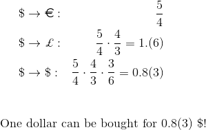
Arbitration is a few logically related transactions aimed at profit from the difference in prices for the same or related assets at the same time in different markets (spatial arbitration), or in the same market at different points in time (temporary arbitration) .

As a simple example, consider spatial arbitrage. In New York and London, deals can be made to buy dollars for euros and euros for dollars. In New York, this can be done at the rate of 4 dollars for 3 euros, and in London - at the rate of 5 dollars for 3 euros. This difference in rates opens up the possibility of spatial arbitration.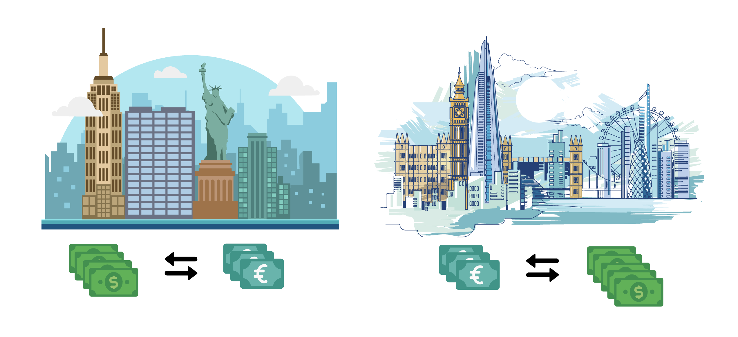



With 4 dollars, in New York you can buy 3 euros. After that, in London, buy for these 3 euros 5 dollars. As you can see, such a simple sequence of transactions brings 1 dollar profit for every 4 dollars invested. Accordingly, if initially there is $ 4 million, then the profit will already be in a million.

When the exchange rates (we do not consider the spread) for the same currency pair differ, the sequence of transactions required to implement the arbitrage strategy is very simple. If the exchange rate for one currency pair is fixed, but several currency pairs are traded in parallel, arbitration is also possible, but the sequence of transactions will already be nontrivial. For example, you can buy 4 euros for 5 dollars, 3 pounds for 4 euros, and then 6 dollars for 3 pounds. The profit from such a sequence of transactions will be $ 1 for every 5 dollars invested.



Hundreds of currency pairs can be traded on the exchange, and exchange rates are constantly changing. It is already impossible to understand what sequence of transactions will bring profit without an algorithmic solution.

Transition to the algorithmic problem

Imagine potential currency exchange transactions in an algorithmic form, namely in the form of a graph. The vertices in this graph represent currencies, and the edges are potential trades. The length of the rib corresponds to the exchange rate at which the transaction can be concluded.


The next question is how to find a sequence of transactions in such a column that will bring profit. Obviously, since at the beginning of the sequence and at the end it must be the same currency, the sequence must correspond to the cycle in the given graph. Next, you need to determine how the exchange rate between the two currencies is calculated if they are not exchanged directly, but through a certain third currency (or an arbitrary number of intermediate operations). Everything here is also quite simple. Such an exchange rate will be calculated as the product of the exchange rates of intermediate transactions. A profitable sequence of transactions becomes if this product takes a value less than one. In other words, if a unit of currency can be bought less than a unit of the same currency.


Classical graph algorithms are poorly suited for working with product of edge lengths. Such algorithms are mainly geared towards finding a path that is defined as the sum of these lengths. However, to circumvent this limitation, there is a mathematical way to go from a product to a sum. This way is logarithm. If the product appears under the logarithm, then such a logarithm can be converted into the sum of the logarithms. On the right side of this equation, the desired number is less than one, which means that the logarithm of this number should be less than zero.




Such a simple mathematical trick allows you to move from searching for a cycle whose product of edge lengths is less than one to finding a cycle whose sum of edge lengths is less than zero. Such a task already looks more solvable by classical graph algorithms, and more precisely the Bellman-Ford algorithm.

Bellman - Ford Algorithm

The Bellman – Ford algorithm is usually used to find the distance from a given vertex to all other vertices of a graph, however, its modification also allows finding cycles of negative length.

The basic operation of this algorithm is edge relaxation . The essence of this operation is as follows. Suppose there is an edge$$$a \ rightarrow b$, and also the previously calculated preliminary values ​​of distances to the peaks are known $$$a$and $$$b$. To perform edge relaxation, it is necessary to calculate what the distance to the top would be$$$b$if the path went through the top $$$a$and rib $$$a \ rightarrow b$. This distance is calculated as the sum of the distance to the top.$$$a$ and rib lengths $$$a \ rightarrow b$. Further, if this distance is less than the current preliminary distance to$$$a$then this is the very distance to $$$a$Corresponds and takes a new, just calculated, value.

The rest of the algorithm is also uncomplicated. Necessary$$$N$ times ($$$N$Is the number of vertices of the graph) bypass the list of edges, applying a relaxation operation for each round. The complexity of the algorithm is obtained$$$N * M$ (Where $$$N$- the number of vertices, and $$$M$- number of ribs). For a graph without negative cycles, further edge relaxation will not lead to a change in the distance to the vertices. At the same time, for a graph containing a negative cycle, relaxation will reduce the distance to the vertices and after$$$N$detours. This property can be used to find the desired cycle.

The following small implementation of the algorithm described above on Kotlin should help those who are more familiar with sorting out code.

fun findNegativeCycle(nodes: Int, edges: Array<Edge>, source: Int): List<Int>? {
    // Initialize distances and prev arrays. All distances but the distance to
    // the source node are infinite, distance to the source node is zero.
    val distances = DoubleArray(nodes) { if (it == source) 0.0 else INFINITY }
    val prev = IntArray(nodes) { -1 }

    // Relax all edges N times where N is the number of nodes.
    repeat(nodes) {
        edges.forEach { it.relax(distances, prev) }
    }

    // Try to relax at least one more edge. If it's possible memorize the node,
    // otherwise return from the method.
    val firstRelaxedEdge = edges.firstOrNull { it.relax(distances, prev) }
    var node = firstRelaxedEdge?.to ?: return null

    // Step back N times where N is the number of nodes. As a result, the node will
    // be in the loop for sure.
    repeat(nodes) {
        node = prev[node]
    }

    // Recover the loop by the node that is inside it and prev links.
    val lastNode = node
    return buildList {
        do {
            add(node)
            node = prev[node]
        } while (node != lastNode)

        reverse()
    }
}

// Edge DTO with implemented relaxation operation.
data class Edge(val from: Int, val to: Int, val length: Double) {

    fun relax(distances: DoubleArray, prev: IntArray): Boolean {
        if (distances[from] + length >= distances[to]) {
            return false
        }

        distances[to] = distances[from] + length
        prev[to] = from
        return true
    }
}

Let us examine an example with a small graph, which includes a cycle of negative length. For the algorithm to work, it is necessary for each vertex to maintain the current known distance to it, as well as a link to its previous vertex. The reference to the previous vertex in this case is determined by the successful relaxation of the rib. If the relaxation operation was successful, and the distance to the vertex was updated, then the link to the previous vertex of this vertex is also updated and takes the value of the source vertex of the specified edge.

So, first you need to initialize the vertices by setting the distance to all the vertices except the initial equal infinity. For the initial vertex, a distance of zero is set.


The first round of all the ribs follows and their relaxation is performed. Almost all relaxation do not give any result, except rib relaxation$$$a \ rightarrow b$. Relaxation of this rib allows you to update the distance to$$$b$.


This is followed by the second round of all edges of the graph and the corresponding relaxation. This time, the result is relaxation of the ribs.$$$b \ rightarrow c$, and $$$b \ rightarrow d$. The distances to the peaks are updated.$$$c$ and $$$d$. It should be noted here that the result depends on the order in which the edges are traversed.


In the third round of ribs, it is possible to successfully relax already three ribs, namely the ribs $$$s \ rightarrow d$, $$$d \ rightarrow e$, $$$d \ rightarrow b$. In this case, when the ribs are relaxed$$$s \ rightarrow d$ and $$$d \ rightarrow b$already recorded distances to $$$d$and $$$b$, as well as corresponding links to previous vertices.


At the fourth round, rib relaxation operations are successfully completed. $$$b \ rightarrow c$and $$$b \ rightarrow a$. In this case, already recorded values ​​of distances to the peaks are again updated.$$$a$ and $$$c$, as well as the corresponding links to previous vertices.


The fifth round is the last. Ribs relax during this walk$$$s \ rightarrow d$, $$$d \ rightarrow b$, $$$d \ rightarrow e$. Here you can see that the presence of a cycle of negative length already makes certain adjustments to the values ​​of distances to the peaks.


After this tour, if the graph did not contain a cycle of negative length, the algorithm would be completed, since the relaxation of any edge would not have made any changes. However, for this graph, due to the presence of a cycle of negative length, one can still find an edge whose relaxation will update the distance to one of the vertices.


An edge whose relaxation updates the distance to the summit is found. This confirms the presence of a cycle of negative length. Now you need to find this cycle itself. It is important that the vertex, the distance to which is now updated, can be both inside the cycle and outside it. In the example, this is the top$$$e$and she is out of cycle. Next, you need to refer to the links to the previous vertices, which were carefully updated at all steps of the algorithm. To be guaranteed to get into the cycle, you must step back on$$$N$peaks using these links.

In this example, the transitions will be as follows:$$$e \ rightarrow d \ rightarrow c \ rightarrow b \ rightarrow d \ rightarrow c$. So the top is located$$$c$, which is guaranteed to lie in a cycle of negative length.


Further, a matter of technology. To return the desired cycle, you need to iterate again using the links to the previous vertices until the vertex meets again$$$c$. This will mean that the cycle has closed. All that remains is to reverse the order, since the iteration was reversed during iterations over links to previous vertices.

The above algorithm assumes the presence of some initial vertex from which the distances are calculated. The presence of such a vertex is not necessary for the algorithm to work, but it was introduced to a greater extent to match the original Bellman - Ford algorithm. If the subject of interest is a cycle of negative length, then we can assume that all the vertices of a given graph are initial. In other words, that the distance to all the vertices is initially zero.

Conclusion

Using the Bellman-Ford algorithm in the arbitrage trading problem is an excellent example of how classical algorithms can solve real business problems, in particular, in the financial sphere. Asymptotic complexity of the algorithm, equal to$$$N ^ 3$for a fully connected graph, it may turn out to be quite large. This really needs to be remembered. However, in many cases, such as currency exchange, this complexity does not create any problems due to the relatively small number of nodes in the graph.