The last article examined how you can get information on financial instruments. Next, several articles will be published on what initially can be done with the data obtained, how to analyze and draw up a strategy. Materials are based on publications in foreign sources and courses on one of the online platforms.This article will discuss how to calculate profitability, volatility and build one of the main indicators.import pandas as pd
import yfinance as yf
import numpy as np
import matplotlib.pyplot as plt
sber = yf.download('SBER.ME','2016-01-01')
Profitability
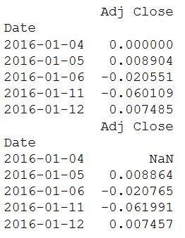
This value represents the percentage change in the value of the stock for one trading day. It does not take into account dividends and commissions. It is easy to calculate using the pct_change () function from the Pandas package.As a rule, log profitability is used, since it allows you to better understand and investigate changes over time.
daily_close = sber[['Adj Close']]
daily_pct_change = daily_close.pct_change()
daily_pct_change.fillna(0, inplace=True)
print(daily_pct_change.head())
daily_log_returns = np.log(daily_close.pct_change()+1)
print(daily_log_returns.head())
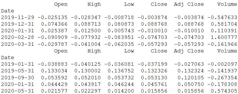
 In order to find out weekly and / or monthly profitability from the obtained data, use the resample () function.
monthly = sber.resample('BM').apply(lambda x: x[-1])
print(monthly.pct_change().tail())
quarter = sber.resample("4M").mean()
print(quarter.pct_change().tail())
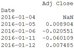
 The pct_change () function is convenient to use, but in turn hides how the value is obtained. A similar calculation that helps to understand the mechanism can be done using shift () from the package from the Pandas package. The daily closing price is divided by the past (shifted by one) price and a unit is subtracted from the received value. But there is one minor minus - the first value as a result is NA.The calculation of profitability is based on the formula:
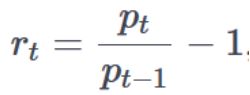 Where, p is the price, t is the time instant and r is the profitability.Next, a profitability distribution diagram is built and the main statistics are calculated:
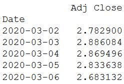
daily_pct_change = daily_close / daily_close.shift(1) - 1
print(daily_pct_change.head())
daily_pct_change.hist(bins=50)
plt.show()
print(daily_pct_change.describe())
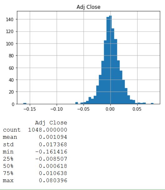 The distribution looks very symmetrical and normally distributed around a value of 0.00. To get other statistics values, the description () function is used. As a result, it is seen that the average value is slightly greater than zero, and the standard deviation is almost 0.02.
Cumulative return
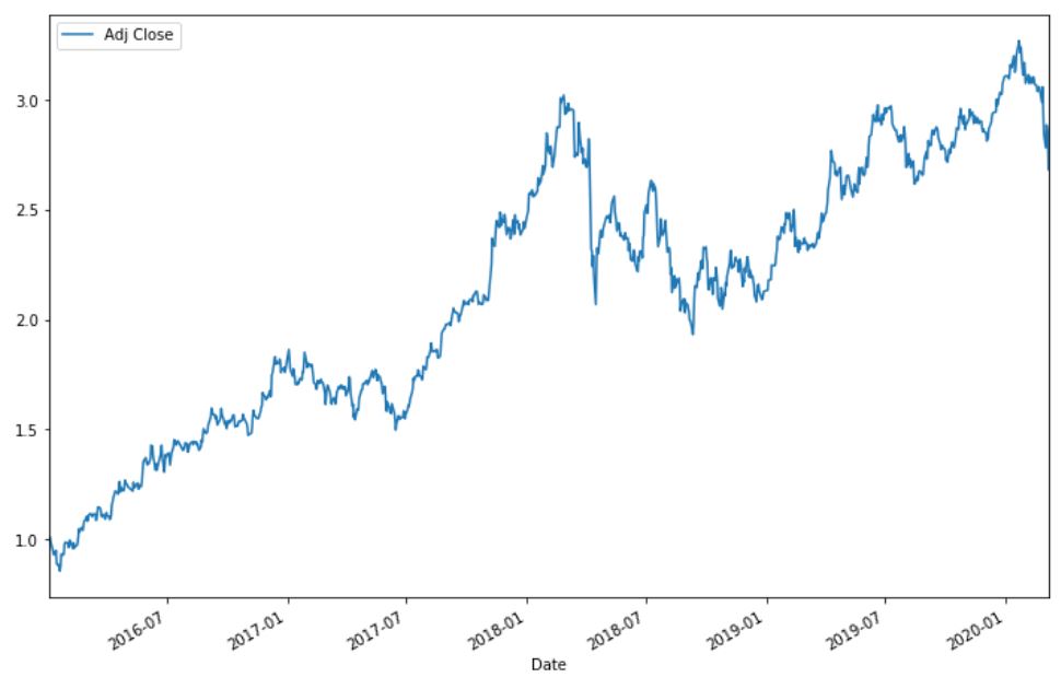
Cumulative daily returns are useful for determining the value of an investment over a specified period of time. It can be calculated as shown in the code below.
cum_daily_return = (1 + daily_pct_change).cumprod()
print(cum_daily_return.tail())
cum_daily_return.plot(figsize=(12,8))
plt.show()
 You can recalculate the yield in the monthly period:
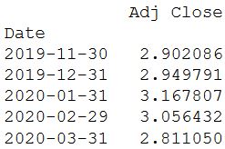
cum_monthly_return = cum_daily_return.resample("M").mean()
print(cum_monthly_return.tail())
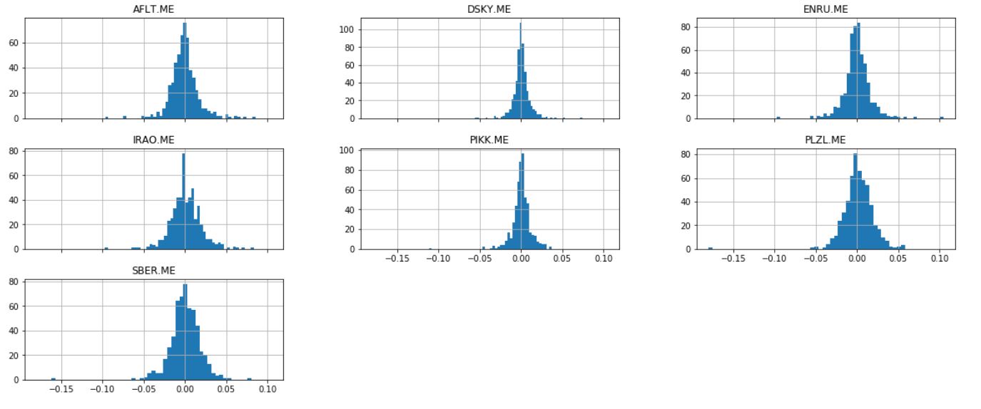
 Knowing how to calculate returns is valuable when analyzing stocks. But it is even more valuable when compared with other stocks.Take some stocks (their choice is completely random) and build their chart.
ticker = ['AFLT.ME','DSKY.ME','IRAO.ME','PIKK.ME', 'PLZL.ME','SBER.ME','ENRU.ME']
stock = yf.download(ticker,'2018-01-01')
daily_pct_change = stock['Adj Close'].pct_change()
daily_pct_change.hist(bins=50, sharex=True, figsize=(20,8))
plt.show()
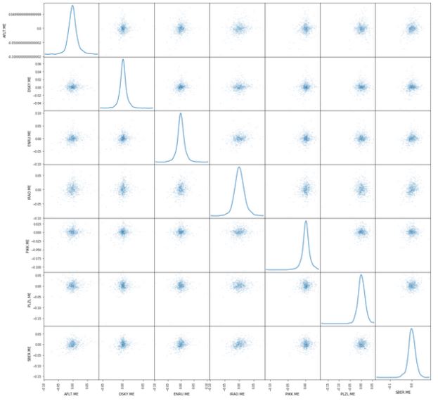
 Another useful graph is the scatter matrix. It can be easily built using the scatter_matrix () function, which is part of the pandas library. Daily_pct_change is used as arguments and the Kernel Density Estimation parameter is set. In addition, you can set the transparency using the alpha parameter and the size of the graph using the figsize parameter.
from pandas.plotting import scatter_matrix
scatter_matrix(daily_pct_change, diagonal='kde', alpha=0.1,figsize=(20,20))
plt.show()
 That's all for now. The next article will cover calculating volatility, average and using the least squares method.