Now programming penetrates deeper and deeper into all areas of life. And maybe it became thanks to the very popular python now. If 5 years ago, for data analysis, you had to use a whole package of various tools: C # for unloading (or pens), Excel, MatLab, SQL, and constantly “jump” there, clearing, verifying and verifying the data. Now python, thanks to a huge number of excellent libraries and modules, in the first approximation safely replaces all these tools, and in conjunction with SQL, in general, “mountains can be rolled up”.So what am I doing. I became interested in learning such a popular python. And the best way to learn something, as you know, is practice. And I'm also interested in real estate. And I came across an interesting problem about real estate in Moscow: to rank Moscow districts by the average rental cost of an average odnushka? Fathers, I thought, here you have geolocation, and uploading from the site, and data analysis - a great practical task.Inspired by the wonderful articles here on Habré (at the end of the article I will add links), let's get started!The task for us is to go through the existing tools inside python, disassemble the technique - how to solve such problems and spend time with pleasure, and not just with benefit.- Scraping Cyan
- Single data frame
- Data frame processing
- results
- A bit about working with geodata
Scraping Cyan
In mid-March 2020, it was possible to collect almost 9 thousand proposals for renting a 1-room apartment in Moscow on cyan, the site displays 54 pages. We will work with jupyter-notebook 6.0.1, python 3.7. We upload data from the site and save it to files using the requests library .So that the site doesn’t ban us, we will disguise ourselves as a person by adding a delay in requests and setting a header so that from the side of the site we look like a very smart person making requests through a browser. Do not forget to check the response from the site each time, otherwise we are suddenly discovered and already banned. You can read more and more detailed about website scraping, for example, here: Web Scraping using python .It’s also convenient to add decorators to evaluate the speed of our functions and logging. Setting level = logging.INFO allows you to specify the type of messages displayed in the log. You can also configure the module to output the log to a text file, for us this is unnecessary.The codedef timer(f):
def wrap_timer(*args, **kwargs):
start = time.time()
result = f(*args, **kwargs)
delta = time.time() - start
print (f' {f.__name__} {delta} ')
return result
return wrap_timer
def log(f):
def wrap_log(*args, **kwargs):
logging.info(f" {f.__doc__}")
result = f(*args, **kwargs)
logging.info(f": {result}")
return result
return wrap_log
logging.basicConfig(level=logging.INFO)
@timer
@log
def requests_site(N):
headers = ({'User-Agent':'Mozilla/5.0 (Macintosh; Intel Mac OS X 10_13_6) AppleWebKit/605.1.15 (KHTML, like Gecko) Version/13.0.5 Safari/605.1.15'})
pages = [106 + i for i in range(N)]
n = 0
for i in pages:
s = f"https://www.cian.ru/cat.php?deal_type=rent&engine_version=2&page={i}&offer_type=flat®ion=1&room1=1&type=-2"
response = requests.get(s, headers = headers)
if response.status_code == 200:
name = f'sheets/sheet_{i}.txt'
with open(name, 'w') as f:
f.write(response.text)
n += 1
logging.info(f" {i}")
else:
print(f" {i} response.status_code = {response.status_code}")
time.sleep(np.random.randint(7,13))
return f" {n} "
requests_site(300)
Single data frame
For scraping pages, choose BeautifulSoup and lxml . We use "beautiful soup" simply for its cool name, although, they say that lxml is faster.You can do it beautifully, take a list of files from a folder using the os library , filter out the extensions we need and go through them. But we will make it easier, since we know the exact number of files and their exact names. Unless we add decoration in the form of a progress bar, using the tqdm libraryThe code
from bs4 import BeautifulSoup
import re
import pandas as pd
from dateutil.parser import parse
from datetime import datetime, date, time

def read_file(filename):
    with open(filename) as input_file:
        text = input_file.read()
    return text

import tqdm

site_texts = []
pages = [1 + i for i in range(309)]

for i in tqdm.tqdm(pages):
    name = f'sheets/sheet_{i}.txt'
    site_texts.append(read_file(name))

print(f" {len(site_texts)} .")

def parse_tag(tag, tag_value, item):
    key = tag
    value = "None"
    if item.find('div', {'class': tag_value}):
        if key == 'link':
            value = item.find('div', {'class': tag_value}).find('a').get('href')
        elif (key == 'price' or key == 'price_meter'):
            value = parse_digits(item.find('div', {'class': tag_value}).text, key)
        elif key == 'pub_datetime':
            value = parse_date(item.find('div', {'class': tag_value}).text)
        else:
            value = item.find('div', {'class': tag_value}).text
    return key, value


def parse_digits(string, type_digit):
    digit = 0
    try:
        if type_digit == 'flats_counts':
            digit = int(re.sub(r" ", "", string[:string.find("")]))
        elif type_digit == 'price':
            digit = re.sub(r" ", "", re.sub(r"₽", "", string))
        elif type_digit == 'price_meter':
            digit = re.sub(r" ", "", re.sub(r"₽/²", "", string))
    except:
        return -1
    return digit

def parse_date(string):
    now = datetime.strptime("15.03.20 00:00", "%d.%m.%y %H:%M")
    s = string
    if string.find('') >= 0:
        s = "{} {}".format(now.day, now.strftime("%b"))
        s = string.replace('', s)
    elif string.find('') >= 0:
        s = "{} {}".format(now.day - 1, now.strftime("%b"))
        s = string.replace('',s)
    if (s.find('') > 0):
        s = s.replace('','mar')
    if (s.find('') > 0):
        s = s.replace('','feb')
    if (s.find('') > 0):
        s = s.replace('','jan')
    return parse(s).strftime('%Y-%m-%d %H:%M:%S')


def parse_text(text, index):

    tag_table = '_93444fe79c--wrapper--E9jWb'
    tag_items = ['_93444fe79c--card--_yguQ', '_93444fe79c--card--_yguQ']
    tag_flats_counts = '_93444fe79c--totalOffers--22-FL'
    tags = {
        'link':('c6e8ba5398--info-section--Sfnx- c6e8ba5398--main-info--oWcMk','undefined c6e8ba5398--main-info--oWcMk'),
        'desc': ('c6e8ba5398--title--2CW78','c6e8ba5398--single_title--22TGT', 'c6e8ba5398--subtitle--UTwbQ'),
        'price': ('c6e8ba5398--header--1df-X', 'c6e8ba5398--header--1dF9r'),
        'price_meter': 'c6e8ba5398--term--3kvtJ',
        'metro': 'c6e8ba5398--underground-name--1efZ3',
        'pub_datetime': 'c6e8ba5398--absolute--9uFLj',
        'address': 'c6e8ba5398--address-links--1tfGW',
        'square': ''
    }

    res = []
    flats_counts = 0
    soup = BeautifulSoup(text)
    if soup.find('div', {'class': tag_flats_counts}):
        flats_counts = parse_digits(soup.find('div', {'class': tag_flats_counts}).text, 'flats_counts')

    flats_list = soup.find('div', {'class': tag_table})
    if flats_list:
        items = flats_list.find_all('div', {'class': tag_items})
        for i, item in enumerate(items):

            d = {'index': index}
            index += 1
            for tag in tags.keys():
                tag_value = tags[tag]
                key, value = parse_tag(tag, tag_value, item)
                d[key] = value
            results[index] = d

    return flats_counts, index

from IPython.display import clear_output

sum_flats = 0
index = 0
results = {}
for i, text in enumerate(site_texts):
    flats_counts, index = parse_text(text, index)
    sum_flats = len(results)
    clear_output(wait=True)
    print(f"  {i + 1} flats = {flats_counts},   {sum_flats} ")
print(f" sum_flats ({sum_flats}) = flats_counts({flats_counts})")
An interesting nuance was that the figure indicated at the top of the page and indicating the total number of apartments found on request differs from page to page. So, in our example, this 5,402 offers are sorted by default, ranging from 5343 to 5402, gradually decreasing with increasing page number of the request (but not by the number of displayed ads). In addition, it was possible to continue to unload pages beyond the limits of the number of pages indicated on the site. In our case, only 54 pages were offered on the site, but we were able to unload 309 pages, with only older ads, for a total of 8640 apartment rental ads.An investigation of this fact will be left outside the scope of this article.Data frame processing
So, we have a single data frame with raw data on 8640 offers. We will conduct a surface analysis of the average and median prices in the districts, calculate the average rental price per square meter of the apartment and the cost of the apartment in the district “on average”.We will proceed from the following assumptions for our study:- Lack of repetitions: all apartments found are truly existing apartments. At the first stage, we eliminated repeated apartments at the address and quadrature, but if the apartment has a slightly different quadrature or address, we consider these options as different apartments.
- — .
— «» ? ( ) , , , , . , , , . «» : . «» ( ) , .
We will need:price_per_month - monthly price rent in rublessquare -okrug area - district, in this study the whole address is not interesting to usprice_meter - rental price per 1 square meterThe codedf['price_per_month'] = df['price'].str.strip('/.').astype(int)
new_desc = df["desc"].str.split(",", n = 3, expand = True)
df["square"]= new_desc[1].str.strip(' ²').astype(int)
df["floor"]= new_desc[2]
new_address = df['address'].str.split(',', n = 3, expand = True)
df['okrug'] = new_address[1].str.strip(" ")
df['price_per_meter'] = (df['price_per_month'] / df['square']).round(2)
df = df.drop(['index','metro', 'price_meter','link', 'price','desc','address','pub_datetime','floor'], axis='columns')
Now we’ll “take care” of emissions manually according to the schedules. To visualize the data, let's look at three libraries: matplotlib , seaborn and plotly .Histograms of data . Matplotlib allows you to quickly and easily display all the charts for the data groups that interest us, we don’t need more. The figure below, according to which only 1 proposal in Mitino cannot serve as a qualitative assessment of the average apartment, is deleted. Another interesting picture in the Southern Administrative Okrug: the majority of offers (more than 500 units) with rental value below 1000 rubles, and a surge in offers (almost 300 units) by 1700 rubles per square meter. In the future, you can see why this happens - rummaging in other indicators for these apartments.Just one line of code gives histograms there for grouped data sets:hists = df['price_per_meter'].hist(by=df['okrug'], figsize=(16, 14), color = "tab:blue", grid = True)
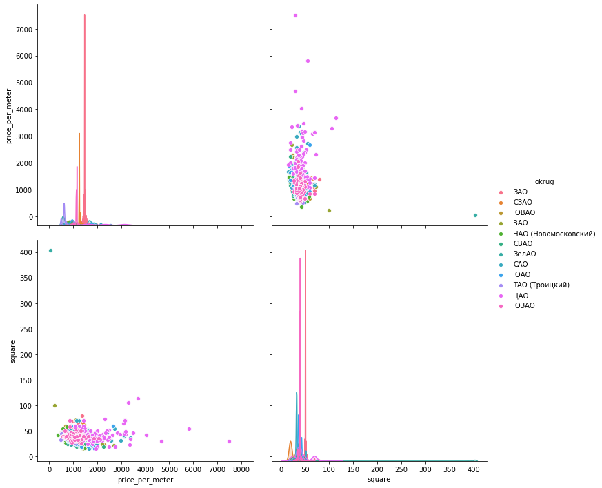
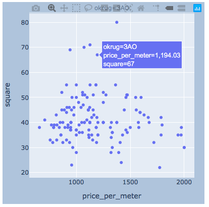
 The scatter of values . Below presented the graphs using all three libraries. seaborn by default is more beautiful and bright, but plotly allows you to immediately display the values when you hover the mouse, which is very convenient for us to select the values of the "outliers" that we will delete.matplotlib
fig, axes = plt.subplots(nrows=4,ncols=3,figsize=(15,15))
for i, (name, group) in enumerate(df_copy.groupby('okrug')):
axes = axes.flatten()
axes[i].scatter(group['price_per_meter'],group['square'], color ='blue')
axes[i].set_title(name)
axes[i].set(xlabel=' 1 ..', ylabel=', 2')
fig.tight_layout()
 seaboarn
sns.pairplot(vars=["price_per_meter","square"], data=df_copy, hue="okrug", height=5)
 plotlyI think there will be enough example for one district.
import plotly.express as px

for i, (name, group) in enumerate(df_copy.groupby('okrug')):
    fig = px.scatter(group, x="price_per_meter", y="square", facet_col="okrug",
                 width=400, height=400)
    fig.update_layout(
        margin=dict(l=20, r=20, t=20, b=20),
        paper_bgcolor="LightSteelBlue",
    )
    fig.show()
results
So, having cleaned the data, expertly removing emissions, we have 8602 “clean” offers.Next, we calculate the main statistics according to the data: average, median, standard deviation, we get the following rating of Moscow districts as the average rental cost for an average apartment decreases: You can draw beautiful histograms by comparing, for example, average and median prices in the district:
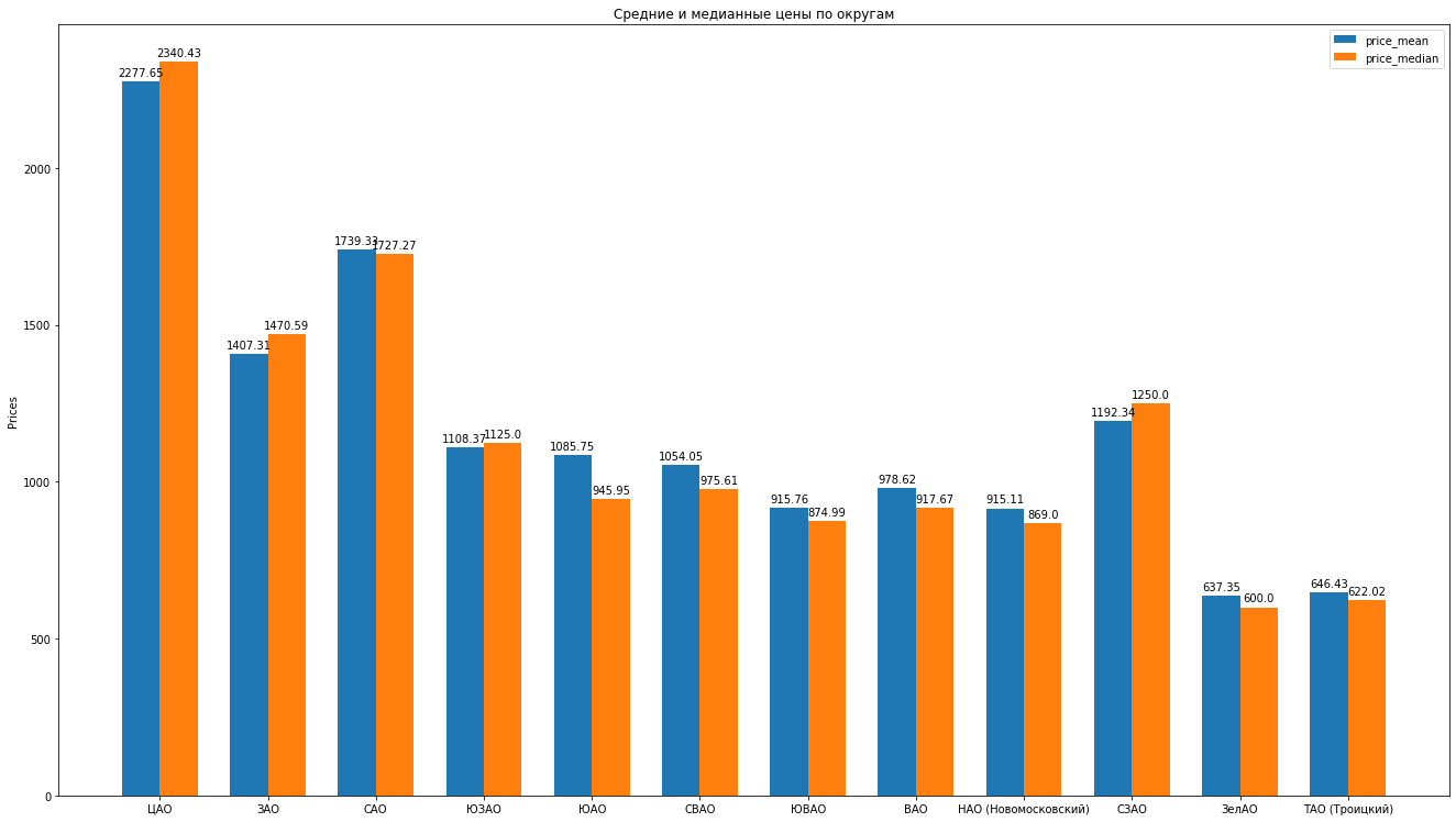 What else can say about the structure of proposals for rental apartments based on data:
- , , , . “” , ( ). , , , , , , “” . , , .
- . . « ». , «» — . . . , , , , , - , , . . .
- , “” , . , , — .
A separate, incredibly interesting and beautiful chapter is the topic of geodata, the display of our data in relation to the map. You can look in very detail and detail, for example, in the following articles:Visualization of election results in Moscow on a map in a Jupyter NotebookLikbez on cartographic projections withOpenStreetMap images as a source of geodataBriefly, OpenStreetMap is our everything, convenient tools are: geopandas , cartoframes (they say it’s already died?) and folium , which we will use.Here's what our data will look like on an interactive map.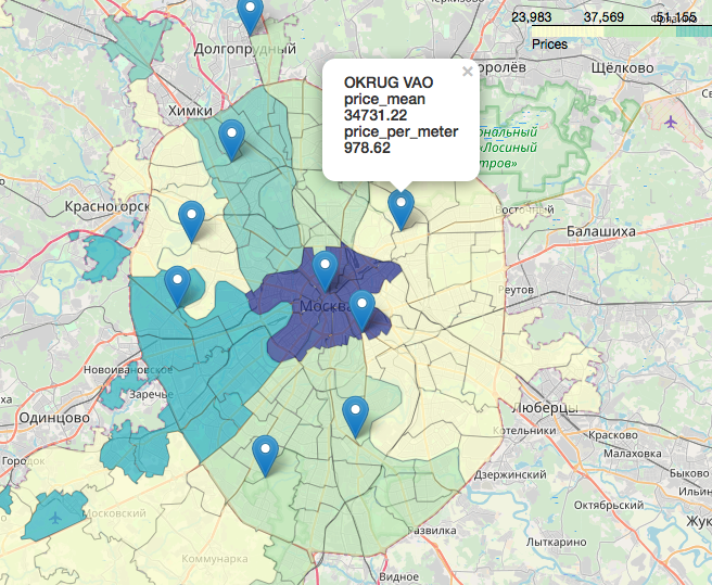 Materials that turned out to be useful in the work on the article:I hope you were interested, like me.Thank you for reading. Constructive criticism is welcome.Sources and datasets are posted on the github here .