哈Ha!今天,我想分享一个如何进行聚类分析的小例子。在此示例中,读者将找不到神经网络和其他流行的方向。该示例可以用作参考点,以便对其他数据进行小型完整的聚类分析。任何有兴趣的人-欢迎猫。
立即提出保留,本文决不声称它是完整的学术性,所获得结果的独特性或对该问题报道的完整性。本文旨在演示经典聚类分析的基本步骤,这些步骤可用于简单而有意义的研究(可能在更详细的研究之前)。欢迎对优点进行任何更正,评论和补充。
该数据是2010年按人均酒精饮料(啤酒,葡萄酒,烈酒等)类型划分的人均酒精消费量(占人均酒精消费量的百分比)的样本。数据还包含:人均每日平均酒精消费量(以纯酒精克为单位)和所有(记录的+未计算出的)人均酒精消费量(仅饮酒者以升纯酒精为单位)。
同时,每个国家有条件地属于以下地理区域之一:东部,中部和西部。由于各种原因,该划分是非常任意的,并且引起争议,但是我们将从现有的角度出发。数据来源-2014年全球酒精与健康状况报告,S。289-364
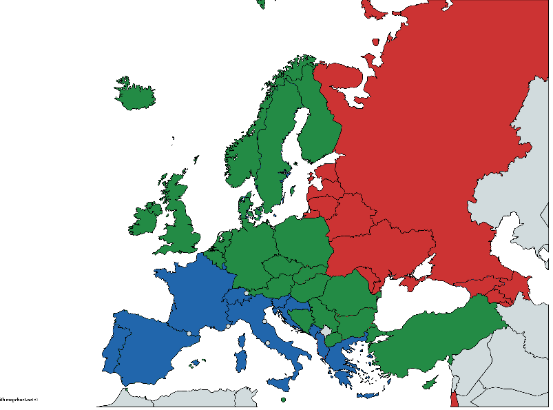
(手绘,可能有错误,但是我认为总体思路是可以理解的)
初步分析
连接使用的库。
library(rgl)
library(heplots)
library(MVN)
library(klaR)
library('Morpho')
library(caret)
library(mclust)
library(ggplot2)
library(GGally)
library(plyr)
library(psych)
library(GPArotation)
library(ggpubr)
, .
#
data <- read.table("alcohol_data.csv", header=TRUE,  sep=",")
#
rownames(data) <- make.names(data[,1], unique = TRUE)
#     ,
data <- data[,-1]
data <- na.omit(data)
#
head(data)
summary(data)
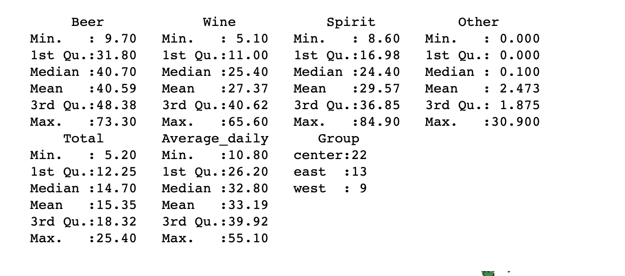
, . , Other , , , , . , , , , . , . - .
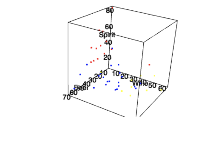
, , , .
options(rgl.useNULL=TRUE)
open3d()
mfrow3d(2,2)
levelColors <- c('west'='blue', 'east'='red', 'center'='yellow')
plot3d(data$Beer, data$Wine, data$Spirit, xlab="Beer", ylab="Wine", zlab="Spirit", col = levelColors[data$Group], size=3)

widget <- rglwidget()
widget
, . , .
ggpairs(
  data,
  mapping = ggplot2::aes(color = data$Group),
  upper = list(continuous = wrap("cor", alpha = 0.5), combo = "box"),
  lower = list(continuous = wrap("points", alpha = 0.3), combo = wrap("dot", alpha = 0.4)),
  diag = list(continuous = wrap("densityDiag",alpha = 0.5)),
  title = "Alcohol"
)
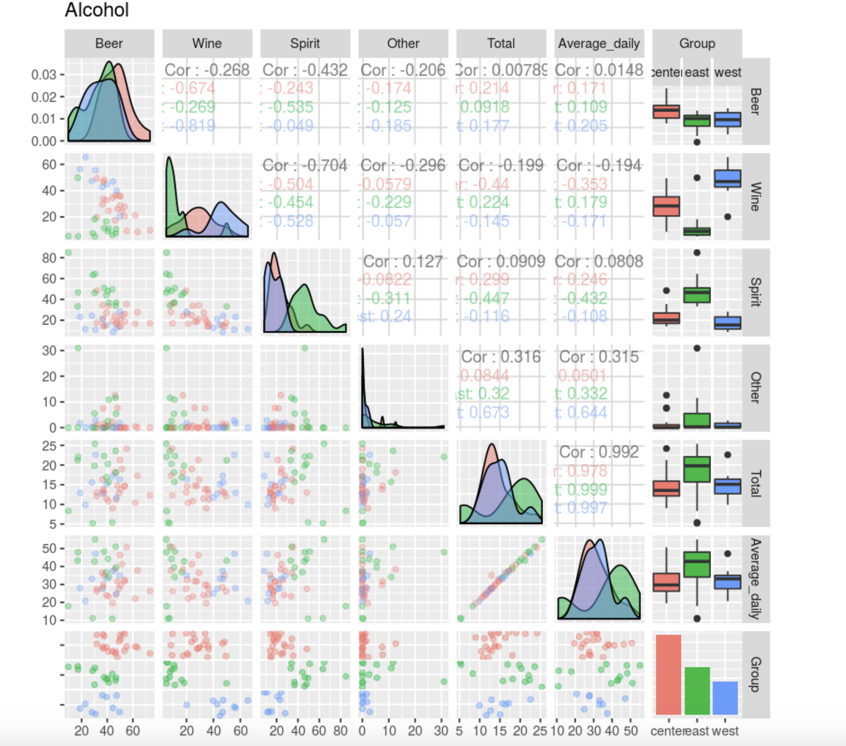
Average Total , Average.
data <- data[, -6]
, , , , . .
data[data$Wine>60,]
, , , , - , , .
data[data$Spirit>70,]
data[data$Spirit<10,]
, , .
,
split(data[,1:5],data$Group)
$center
$east
$west
ggpairs(
  data,
  mapping = ggplot2::aes(color = data$Group),
  diag=list(continuous="bar", alpha=0.4)
)
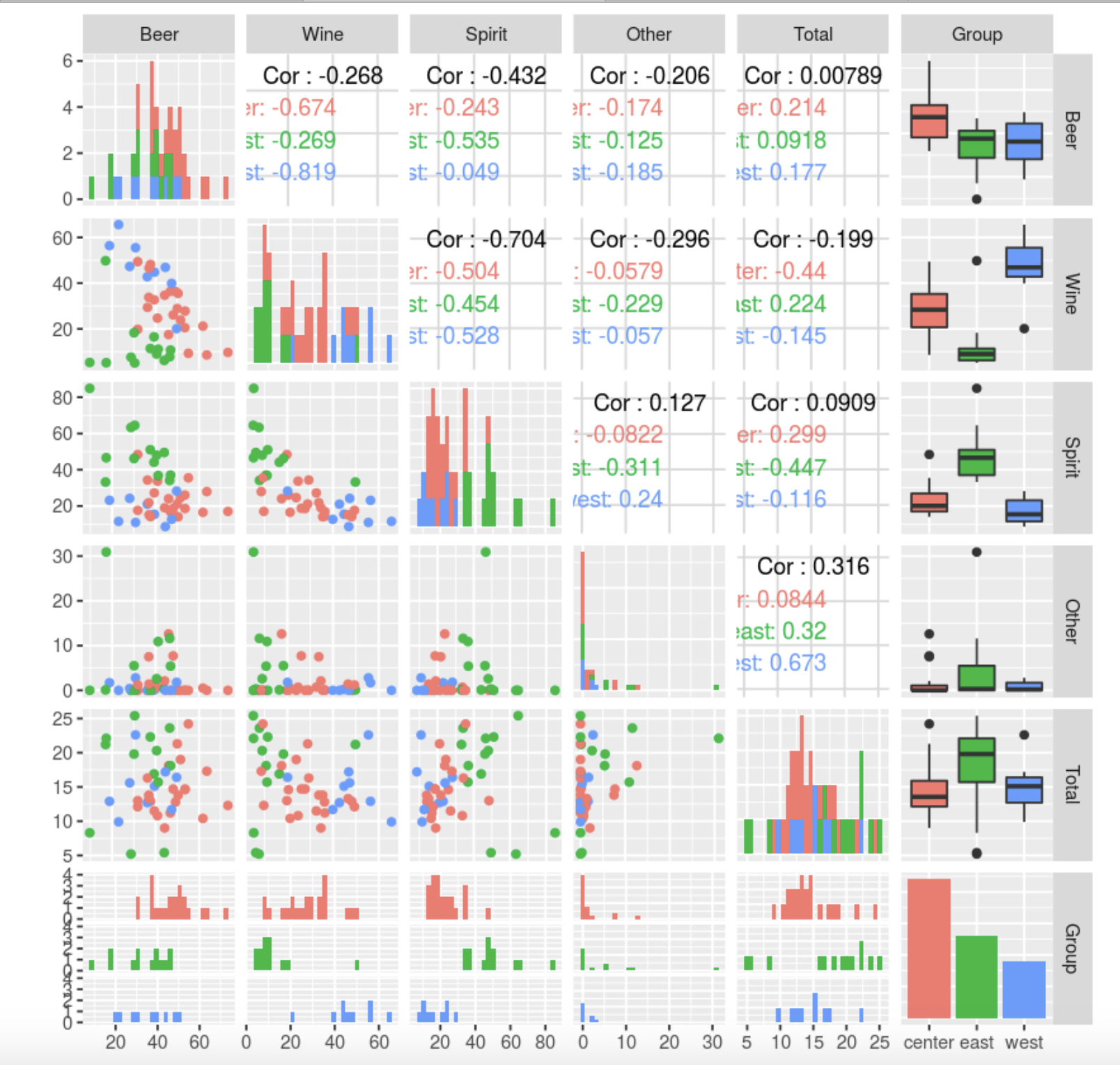
, , . Other, : , , , ( 10-12 , 45, , ). . , , , (). , , . Other .
, , — , — . , — , .
Total Other, . .
, Beer, Spirit Wine . , , , . , , , , , .
Total. , — .
data.group = data[,5]
data <- data[,-5]
data<- data[,-4]
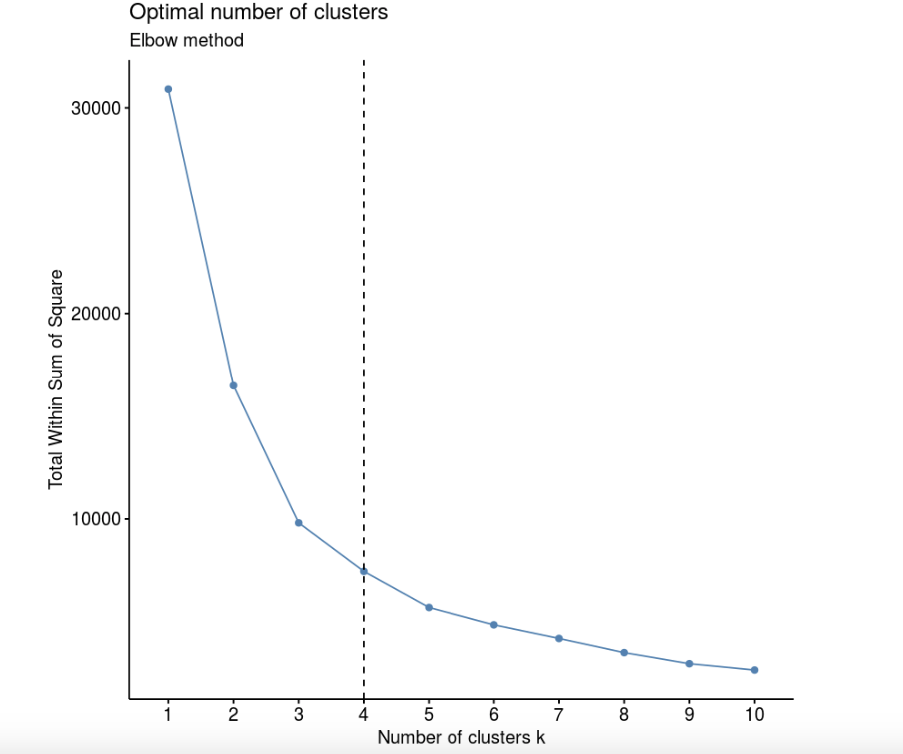
Elbow method (“ ”, “ ”). , k, – W(K), .
library(factoextra)
fviz_nbclust(data, kmeans, method = "wss") +
  labs(subtitle = "Elbow method") +
  geom_vline(xintercept = 4, linetype = 2)
data.dist <- dist((data))
hc <- hclust(data.dist, method = "ward.D2")
plot(hc, cex = 0.7)
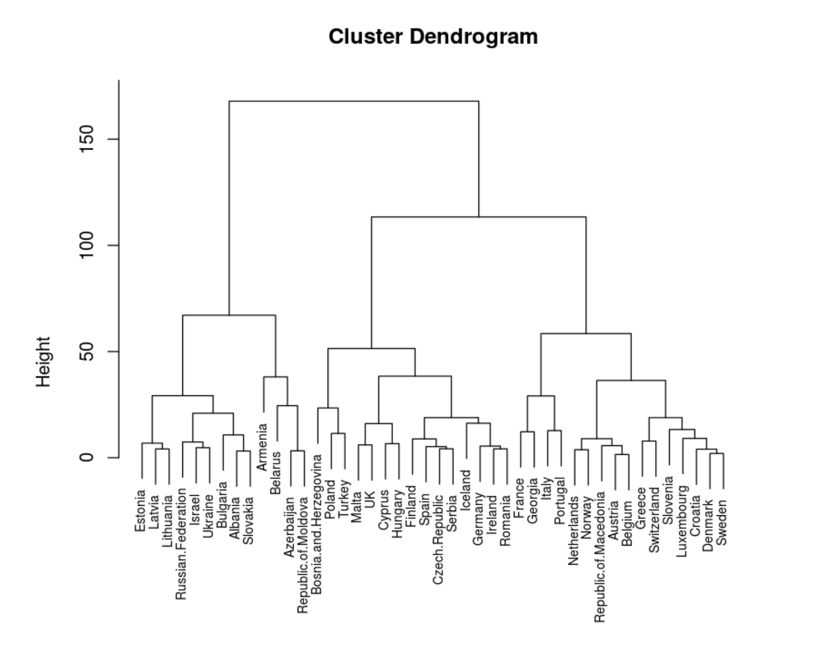
. .
colors=c('green', 'red', 'blue')
hcd = as.dendrogram(hc)
clusMember = cutree(hc, 4)
colLab <- function(n) {
    if (is.leaf(n)) {
        a <- attributes(n)
        labCol <- colors[data.group[n]]
        attr(n, "nodePar") <- c(a$nodePar, lab.col = labCol)
    }
    n
}
clusDendro = dendrapply(hcd, colLab)
plot(clusDendro, main = "Cool Dendrogram", type = "triangle")

rect.hclust(hc, k = 4)
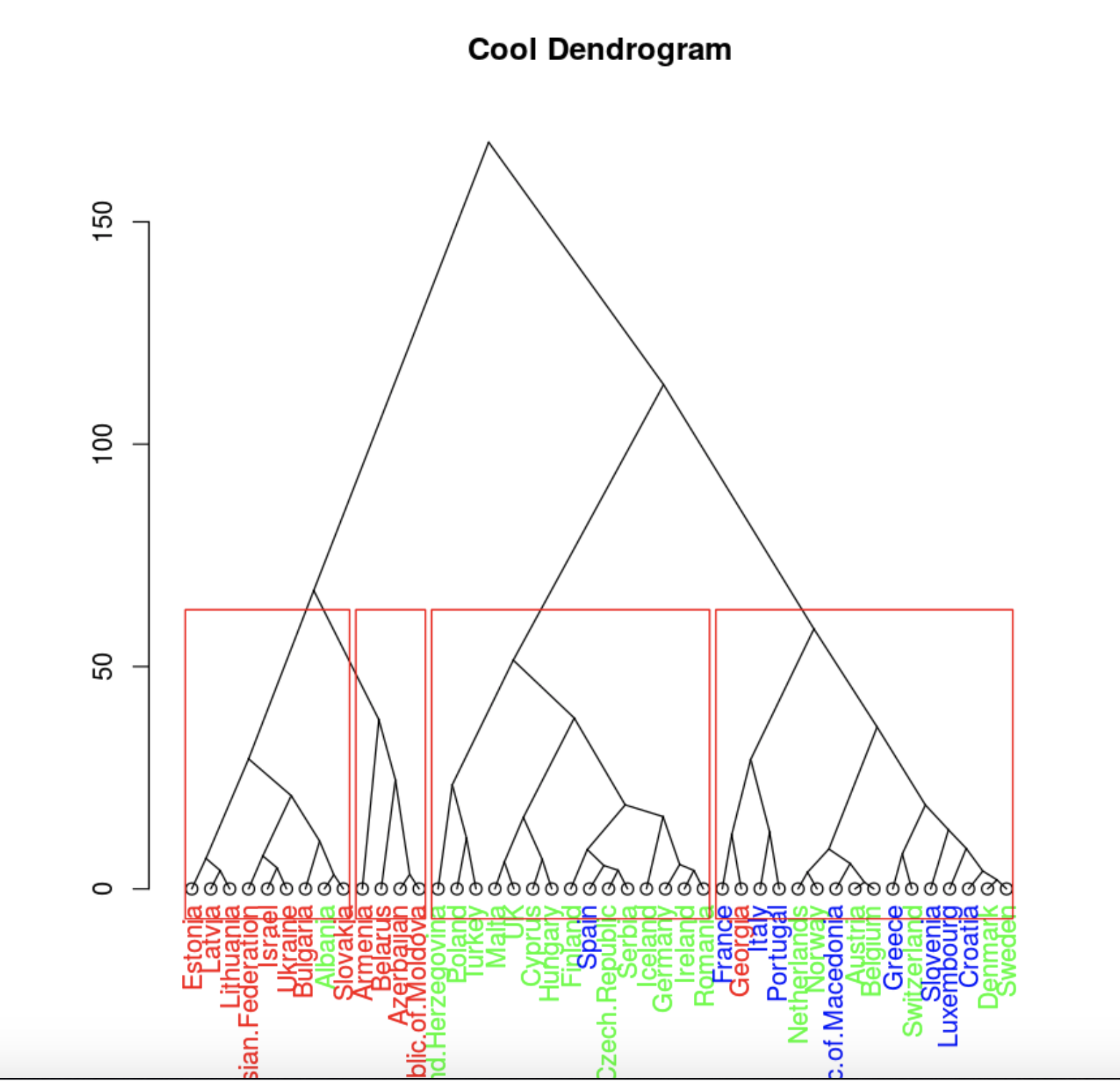
. , .
, , , 4 .
plot(clusDendro, main = "Cool Dendrogram", type = "triangle")
data.hclas_group <- factor(cutree(hc, k = 3))

rect.hclust(hc, k = 3)
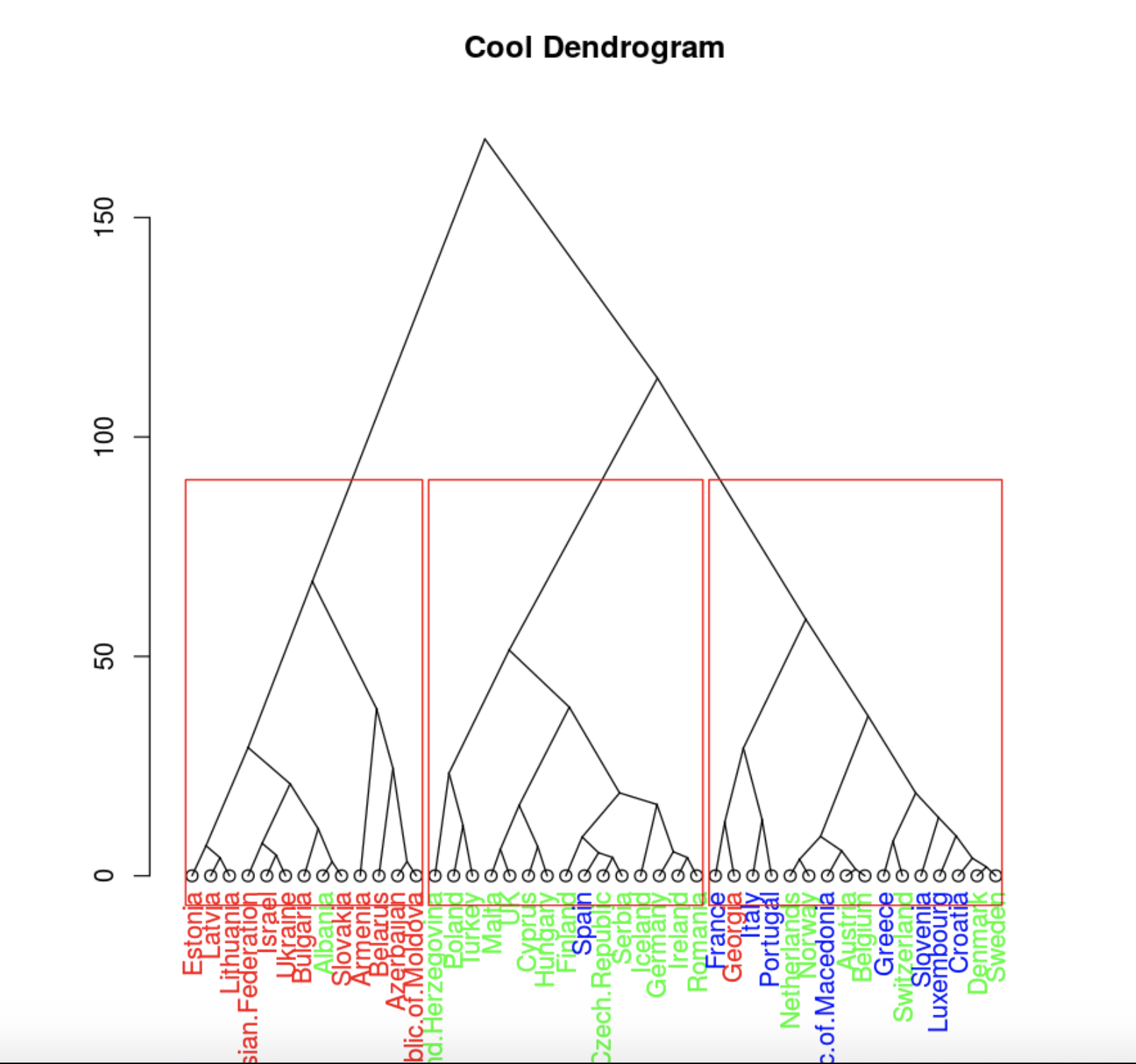
, , .
library(FactoMineR)
res.pca <- PCA(data,scale.unit=T, graph = F)
fviz_pca_biplot(res.pca,
                col = colors[data.hclas_group], palette = "jco",
                label = "var",
                ellipse.level = 0.8,
                 addEllipses = T,
                col.var = "black",
                legend.title = "groups4")
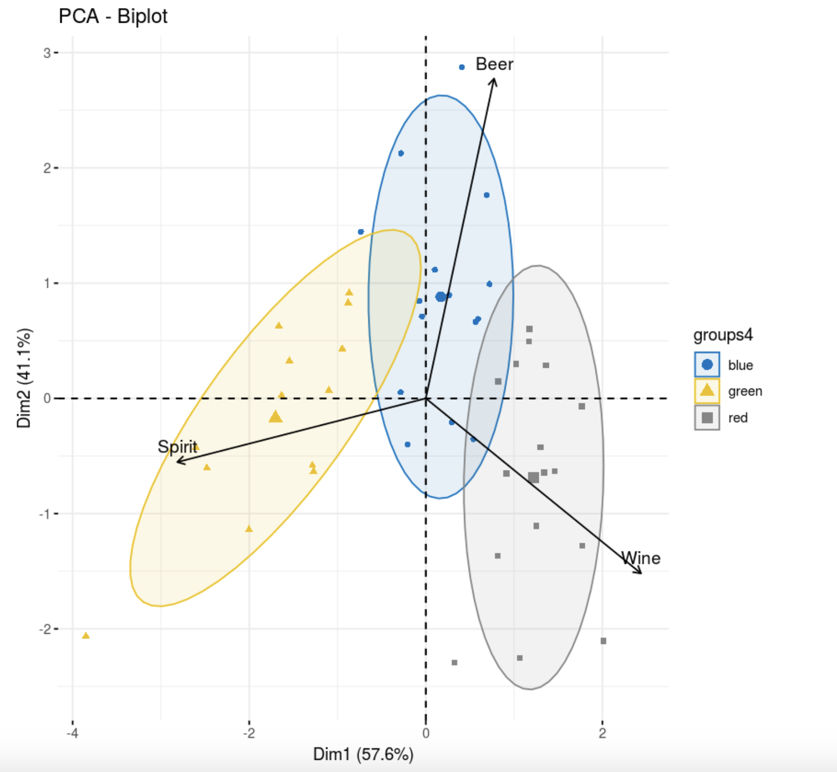
, , . , , , , . , , , k-++.
library(flexclust)
data.kk <- kcca(data, k=3, family=kccaFamily("kmeans"),
control=list(initcent="kmeanspp"))

fviz_pca_biplot(res.pca,
                col.ind =as.factor(data.kk@cluster), palette = "jco",
                label = "var",
                ellipse.level = 0.8,
                 addEllipses = T,
                col.var = "black", repel = TRUE,
                legend.title = "clusters")
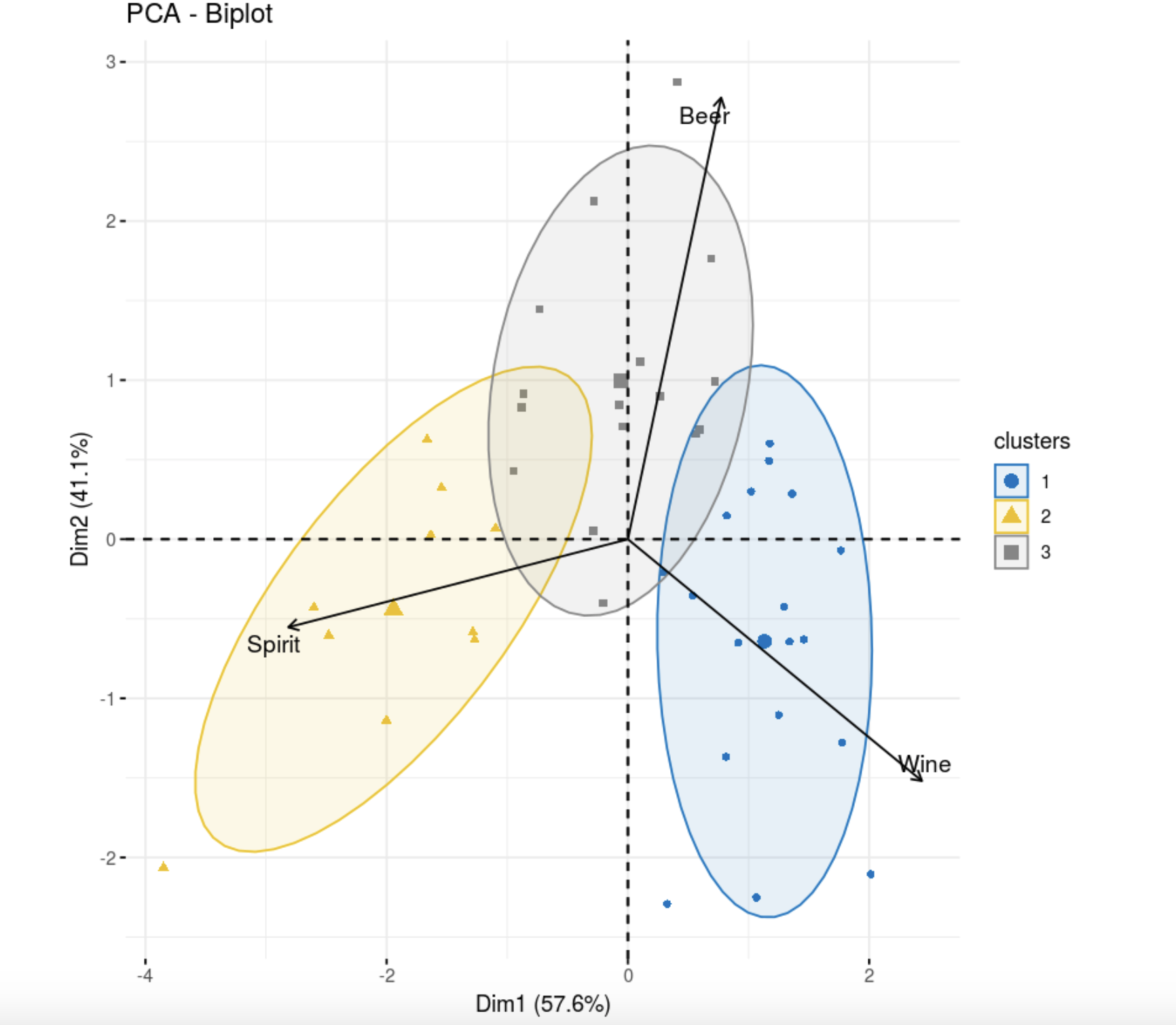
, k- . , , .
, , hclust. .
, , . . , .
. . , , , . , , . , .
可以使用信息标准(此处为描述)基于聚类模型的假设进行聚类,也可以尝试对该数据集进行经典判别分析。如果这篇文章有用,我计划出版续集。