任何活动都会生成数据。无论您做什么,都可能拥有原始有用信息的仓库,或者至少可以访问其来源。
今天的赢家是根据客观数据做出决策的人。分析人员的技能比以往任何时候都更加重要,并且可用的必要工具使您始终领先一步。这有助于本文的外观。
你有自己的生意吗?也许……不过,没关系。数据挖掘的过程是无穷无尽的。即使只是很好地在Internet上进行挖掘,您也可以找到一个活动领域。
这就是我们今天拥有的 -RuTracker.ORG 的非正式XML分发数据库。该数据库每六个月更新一次,其中包含有关该洪流跟踪器存在的历史的所有分布的信息。
她能告诉rutracker的主人什么?以及互联网上盗版的直接帮凶?还是喜欢动漫的普通用户?
你明白我的意思吗?
堆栈-R,Clickhouse,Dataiku
任何分析都经历几个主要阶段:数据提取,准备和数据研究(可视化)。每个阶段都有自己的工具。因为今天的堆栈:
- R.是的,不受欢迎且不如Python。但是它的dplyr和ggplot2仍然干净漂亮。他为分析而生,不使用它是犯罪。
- Clickhouse。柱分析DBMS。可以肯定地说:“ Clickhouse不会减慢速度”或“快到小说的边缘”。人们没有撒谎,我们将看到这一点。负责即时性。
- 达蒂库 用于处理,可视化和预测分析业务数据的平台。
评论: Dataiku在Linux和Mac上运行。一个免费版本可用,最多可容纳3人。文档在这里。
令人惊讶的是,如果您愿意的话,此平台在俄语语言资源甚至在哈布雷(Habré)上的不可抗拒性都没有大肆宣传。我将纠正这种误解,并请您对dataiku的举措表示祝贺。
大数据-大问题
xml– 5 . – rutracker.org, (2005 .) 2019 . 15 !
R Studio – ! . , .
, R. Big Data, Clickhouse … , xml–. . .
. Dataiku DSS . – 10 000 . . , . , 200 000 .
, . .

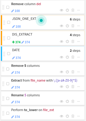
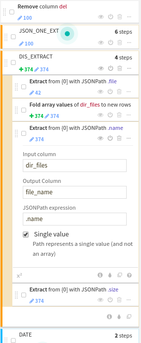
. : content — json.
content, . – .
recipe — . , . json .
. , , + dataiku.
recipe, — .
csv Clickhouse.
Clickhouse 15 rutracker-a.
?
SELECT ROUND(uniq(torrent_id) / 1000000, 2) AS Count_M
FROM rutracker

┌─Count_M─┐
│    1.46 │
└─────────┘
1 rows in set. Elapsed: 0.247 sec. Processed 25.51 million rows, 204.06 MB (103.47 million rows/s., 827.77 MB/s.)
1.5 25 . 0.3 ! .
, , .
SELECT COUNT(*) AS Count
FROM rutracker
WHERE (file_ext = 'epub') OR (file_ext = 'fb2') OR (file_ext = 'mobi')

┌──Count─┐
│ 333654 │
└────────┘
1 rows in set. Elapsed: 0.435 sec. Processed 25.51 million rows, 308.79 MB (58.64 million rows/s., 709.86 MB/s.)
300 — ! , . .
SELECT ROUND(SUM(file_size) / 1000000000, 2) AS Total_size_GB
FROM rutracker
WHERE (file_ext = 'epub') OR (file_ext = 'fb2') OR (file_ext = 'mobi')

┌─Total_size_GB─┐
│        625.75 │
└───────────────┘
1 rows in set. Elapsed: 0.296 sec. Processed 25.51 million rows, 344.32 MB (86.24 million rows/s., 1.16 GB/s.)
– 25 . , ?
R
R. , DBI ( ). Clickhouse.
Rlibrary(DBI) # , ... Clickhouse
library(dplyr) # %>%
#
library(ggplot2)
library(ggrepel)
library(cowplot)
library(scales)
library(ggrepel)
# localhost:9000
connection <- dbConnect(RClickhouse::clickhouse(), host="localhost", port = 9000)
, . dplyr .
? rutracker.org .
Ryears_stat <- dbGetQuery(connection,
"SELECT
round(COUNT(*)/1000000, 2) AS Files,
round(uniq(torrent_id)/1000, 2) AS Torrents,
toYear(torrent_registred_at) AS Year
FROM rutracker
GROUP BY Year")
ggplot(years_stat, aes(as.factor(Year), as.double(Files))) +
geom_bar(stat = 'identity', fill = "darkblue", alpha = 0.8)+
theme_minimal() +
labs(title = " RuTracker", subtitle = " 2005 - 2019\n")+
theme(axis.text.x = element_text(angle=90, vjust = 0.5),
axis.text.y = element_text(),
axis.title.y = element_blank(),
axis.title.x = element_blank(),
panel.grid.major.x = element_blank(),
panel.grid.major.y = element_line(size = 0.9),
panel.grid.minor.y = element_line(size = 0.4),
plot.title = element_text(vjust = 3, hjust = 0, family = "sans", size = 16, color = "#101010", face = "bold"),
plot.caption = element_text(vjust = 3, hjust = 0, family = "sans", size = 12, color = "#101010", face = "bold"),
plot.margin = unit(c(1,0.5,1,0.5), "cm"))+
scale_y_continuous(labels = number_format(accuracy = 1, suffix = " "))
ggplot(years_stat, aes(as.factor(Year), as.integer(Torrents))) +
geom_bar(stat = 'identity', fill = "#008b8b", alpha = 0.8)+
theme_minimal() +
labs(title = " RuTracker", subtitle = " 2005 - 2019\n", caption = "* ")+
theme(axis.text.x = element_text(angle=90, vjust = 0.5),
axis.text.y = element_text(),
axis.title.y = element_blank(),
axis.title.x = element_blank(),
panel.grid.major.x = element_blank(),
panel.grid.major.y = element_line(size = 0.9),
panel.grid.minor.y = element_line(size = 0.4),
plot.title = element_text(vjust = 3, hjust = 0, family = "sans", size = 16, color = "#101010", face = "bold"),
plot.caption = element_text(vjust = -3, hjust = 1, family = "sans", size = 9, color = "grey60", face = "plain"),
plot.margin = unit(c(1,0.5,1,0.5), "cm")) +
scale_y_continuous(labels = number_format(accuracy = 1, suffix = " "))
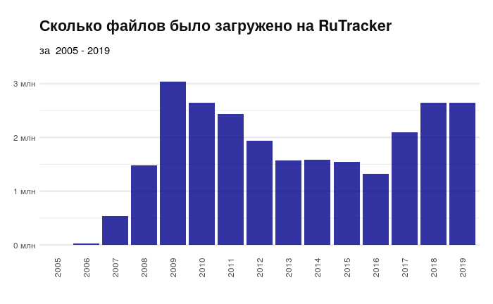
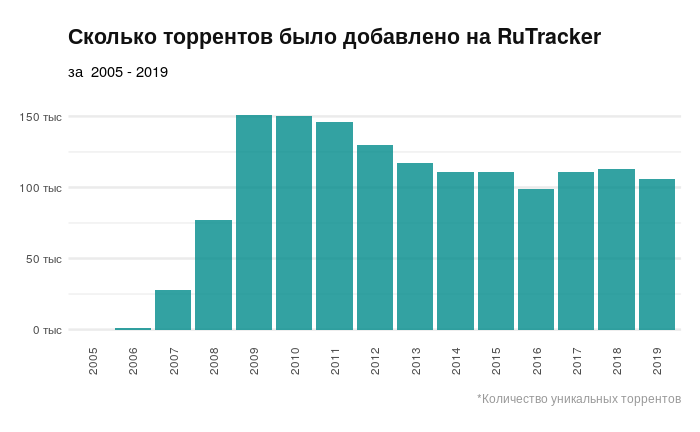
2016 . , 2016 rutracker.org . , .
, . , .
.
Rextention_stat <- dbGetQuery(connection,
"SELECT toYear(torrent_registred_at) AS Year,
COUNT(tracker_id)/1000 AS Count,
ROUND(SUM(file_size)/1000000000000, 2) AS Total_Size_TB,
file_ext
FROM rutracker
GROUP BY Year, file_ext
ORDER BY Year, Count")
#
TopExt <- function(x, n) {
res_tab <- NULL
# 2005 2006, ..
for (i in (3:15)) {
res_tab <-bind_rows(list(res_tab,
extention_stat %>% filter(Year == x[i]) %>%
arrange(desc(Count), desc(Total_Size_TB)) %>%
head(n)
))
}
return(res_tab)
}
years_list <- unique(extention_stat$Year)
ext_data <- TopExt(years_list, 5)
ggplot(ext_data, aes(as.factor(Year), as.integer(Count), fill = file_ext)) +
geom_bar(stat = "identity",position="dodge2", alpha =0.8, width = 1)+
theme_minimal() +
labs(title = " RuTracker",
subtitle = " 2005 - 2019\n",
caption = "* -5 ", fill = "") +
theme(axis.text.x = element_text(angle=90, vjust = 0.5),
axis.text.y = element_text(),
axis.title.y = element_blank(),
axis.title.x = element_blank(),
panel.grid.major.x = element_blank(),
panel.grid.major.y = element_line(size = 0.9),
panel.grid.minor.y = element_line(size = 0.4),
legend.title = element_text(vjust = 1, hjust = -1, family = "sans", size = 9, color = "#101010", face = "plain"),
legend.position = "top",
plot.title = element_text(vjust = 3, hjust = 0, family = "sans", size = 16, color = "#101010", face = "bold"),
plot.caption = element_text(vjust = -4, hjust = 1, family = "sans", size = 9, color = "grey60", face = "plain"),
plot.margin = unit(c(1,0.5,1,0.5), "cm")) +
scale_y_continuous(labels = number_format(accuracy = 0.5, scale = (1/1000), suffix = " "))+guides(fill=guide_legend(nrow=1))
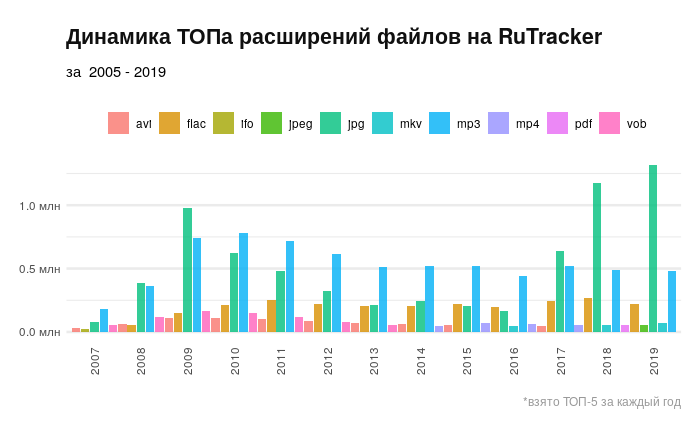
. . .
rutracker-a. .
Rchapter_stat <- dbGetQuery(connection,
"SELECT
substring(forum_name, 1, position(forum_name, ' -')) Chapter,
uniq(torrent_id) AS Count,
ROUND(median(file_size)/1000000, 2) AS Median_Size_MB,
ROUND(max(file_size)/1000000000) AS Max_Size_GB,
ROUND(SUM(file_size)/1000000000000) AS Total_Size_TB
FROM rutracker WHERE Chapter NOT LIKE('\"%')
GROUP BY Chapter
ORDER BY Count DESC")
chapter_stat$Count <- as.integer(chapter_stat$Count)
#
AggChapter2 <- function(Chapter){
var_ch <- str(Chapter)
res = NULL
for(i in (1:22)){
select_str <-paste0(
"SELECT
toYear(torrent_registred_at) AS Year,
substring(forum_name, 1, position(forum_name, ' -')) Chapter,
uniq(torrent_id)/1000 AS Count,
ROUND(median(file_size)/1000000, 2) AS Median_Size_MB,
ROUND(max(file_size)/1000000000,2) AS Max_Size_GB,
ROUND(SUM(file_size)/1000000000000,2) AS Total_Size_TB
FROM rutracker
WHERE Chapter LIKE('", Chapter[i], "%')
GROUP BY Year, Chapter
ORDER BY Year")
res <-bind_rows(list(res, dbGetQuery(connection, select_str)))
}
return(res)
}
chapters_data <- AggChapter2(chapter_stat$Chapter)
chapters_data$Chapter <- as.factor(chapters_data$Chapter)
chapters_data$Count <- as.numeric(chapters_data$Count)
chapters_data %>% group_by(Chapter)%>%
ggplot(mapping = aes(x = reorder(Chapter, Total_Size_TB), y = Total_Size_TB))+
geom_bar(stat = "identity", fill="darkblue", alpha =0.8)+
theme(panel.grid.major.x = element_line(colour="grey60", linetype="dashed"))+
xlab('\n') + theme_minimal() +
labs(title = "C RuTracker-",
subtitle = " 2019\n")+
theme(axis.text.x = element_text(),
axis.text.y = element_text(family = "sans", size = 9, color = "#101010", hjust = 1, vjust = 0.5),
axis.title.y = element_text(vjust = 2.5, hjust = 0, family = "sans", size = 9, color = "grey40", face = "plain"),
axis.title.x = element_blank(),
axis.line.x = element_line(color = "grey60", size = 0.1, linetype = "solid"),
panel.grid.major.y = element_blank(),
panel.grid.major.x = element_line(size = 0.7, linetype = "solid"),
panel.grid.minor.x = element_line(size = 0.4, linetype = "solid"),
plot.title = element_text(vjust = 3, hjust = 1, family = "sans", size = 16, color = "#101010", face = "bold"),
plot.subtitle = element_text(vjust = 2, hjust = 1, family = "sans", size = 12, color = "#101010", face = "plain"),
plot.caption = element_text(vjust = -3, hjust = 1, family = "sans", size = 9, color = "grey60", face = "plain"),
plot.margin = unit(c(1,0.5,1,0.5), "cm"))+
scale_y_continuous(labels = number_format(accuracy = 1, suffix = " "))+
coord_flip()
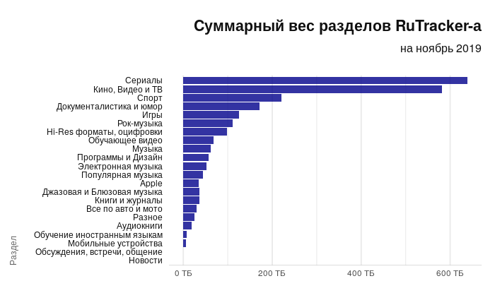
. — — . , . , Apple.
Rchapters_data %>% group_by(Chapter)%>%
ggplot(mapping = aes(x = reorder(Chapter, Count), y = Count))+
geom_bar(stat = "identity", fill="#008b8b", alpha =0.8)+
theme(panel.grid.major.x = element_line(colour="grey60", linetype="dashed"))+
xlab('') + theme_minimal() +
labs(title = " RuTracker-",
subtitle = " 2019\n")+
theme(axis.text.x = element_text(),
axis.text.y = element_text(family = "sans", size = 9, color = "#101010", hjust = 1, vjust = 0.5),
axis.title.y = element_text(vjust = 3.5, hjust = 0, family = "sans", size = 9, color = "grey40", face = "plain"),
axis.title.x = element_blank(),
axis.line.x = element_line(color = "grey60", size = 0.1, linetype = "solid"),
panel.grid.major.y = element_blank(),
panel.grid.major.x = element_line(size = 0.7, linetype = "solid"),
panel.grid.minor.x = element_line(size = 0.4, linetype = "solid"),
plot.title = element_text(vjust = 3, hjust = 1, family = "sans", size = 16, color = "#101010", face = "bold"),
plot.subtitle = element_text(vjust = 2, hjust = 1, family = "sans", size = 12, color = "#101010", face = "plain"),
plot.caption = element_text(vjust = -3, hjust = 1, family = "sans", size = 9, color = "grey60", face = "plain"),
plot.margin = unit(c(1,0.5,1,0.5), "cm"))+
scale_y_continuous(limits = c(0, 300), labels = number_format(accuracy = 1, suffix = " "))+
coord_flip()
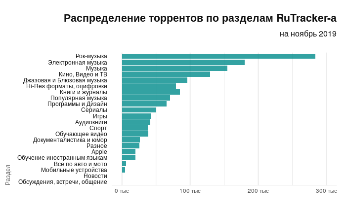
, , : -.
~15 .
Rlibrary("RColorBrewer")
getPalette = colorRampPalette(brewer.pal(19, "Spectral"))
chapters_data %>% #filter(Chapter %in% chapter_stat$Chapter[c(4,6,7,9:20)])%>%
filter(!Chapter %in% chapter_stat$Chapter[c(16, 21, 22)])%>%
filter(Year>=2007)%>%
ggplot(mapping = aes(x = Year, y = Count, fill = as.factor(Chapter)))+
geom_area(alpha =0.8, position = "fill")+
theme_minimal() +
labs(title = " -",
subtitle = " ~15 ", fill = "")+
theme(axis.text.x = element_text(vjust = 0.5),
axis.text.y = element_blank(),
axis.title.y = element_blank(),
axis.title.x = element_blank(),
panel.grid.major.x = element_blank(),
panel.grid.major.y = element_line(size = 0.9),
panel.grid.minor.y = element_line(size = 0.4),
plot.title = element_text(vjust = 3, hjust = 0, family = "sans", size = 16, color = "#101010", face = "bold"),
plot.caption = element_text(vjust = -3, hjust = 1, family = "sans", size = 9, color = "grey60", face = "plain"),
plot.margin = unit(c(1,1,1,1), "cm")) +
scale_x_continuous(breaks = c(2008, 2010, 2012, 2014, 2016, 2018),expand=c(0,0)) +
scale_fill_manual(values = getPalette(19))
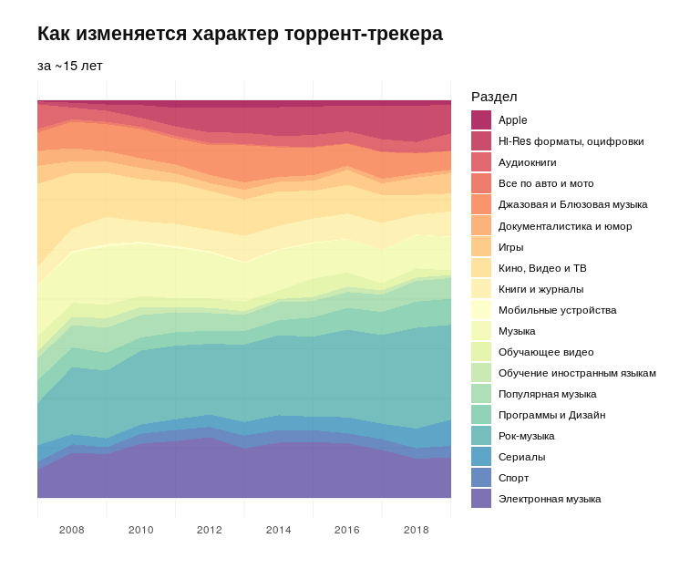
- — . — Apple , .
. .
, Rutracker-a. - rutracker.org.
Runique_torr_per_day <- dbGetQuery(connection,
"SELECT toDate(torrent_registred_at) AS date,
uniq(torrent_id) AS count
FROM rutracker
GROUP BY date
ORDER BY date")
unique_torr_per_day %>%
ggplot(aes(format(date, "%Y"), format(date, "%j"), fill = as.numeric(count)))+
geom_tile() +
theme_minimal() +
labs(title = " RuTracker-a",
subtitle = " ~15 \n\n",
fill = "- \n")+
theme(axis.text.x = element_text(vjust = 0.5),
axis.text.y = element_text(),
axis.title.y = element_blank(),
axis.title.x = element_blank(),
panel.grid.major.y = element_blank(),
panel.grid.major.x = element_line(size = 0.9),
panel.grid.minor.x = element_line(size = 0.4),
legend.title = element_text(vjust = 0.7, hjust = -1, family = "sans", size = 10, color = "#101010", face = "plain"),
legend.position = c(0.88, 1.30),
legend.direction = "horizontal",
plot.title = element_text(vjust = 3, hjust = 0, family = "sans", size = 16, color = "#101010", face = "bold"),
plot.caption = element_text(vjust = -3, hjust = 1, family = "sans", size = 9, color = "grey60", face = "plain"),
plot.margin = unit(c(1,1,1,1), "cm"))+ coord_flip(clip = "off") +
scale_y_discrete(breaks = c(format(as.Date("2007-01-15"), "%j"),
format(as.Date("2007-02-15"), "%j"),
format(as.Date("2007-03-15"), "%j"),
format(as.Date("2007-04-15"), "%j"),
format(as.Date("2007-05-15"), "%j"),
format(as.Date("2007-06-15"), "%j"),
format(as.Date("2007-07-15"), "%j"),
format(as.Date("2007-08-15"), "%j"),
format(as.Date("2007-09-15"), "%j"),
format(as.Date("2007-10-15"), "%j"),
format(as.Date("2007-11-15"), "%j"),
format(as.Date("2007-12-15"), "%j")),
labels = c("", "", "", "", "", "","", "", "", "","",""), position = 'right') +
scale_fill_gradientn(colours = c("#155220", "#c6e48b")) +
annotate(geom = "curve", x = 16.5, y = 119, xend = 13, yend = 135,
curvature = .3, color = "grey15", arrow = arrow(length = unit(2, "mm"))) +
annotate(geom = "text", x = 16, y = 45,
label = " « » \n",
hjust = "left", vjust = -0.75, color = "grey25") +
guides(x.sec = guide_axis_label_trans(~.x)) +
annotate("rect", xmin = 11.5, xmax = 12.5, ymin = 1, ymax = 366,
alpha = .0, colour = "white", size = 0.1) +
geom_segment(aes(x = 11.5, y = 25, xend = 12.5, yend = 25, colour = "segment"),
show.legend = FALSE)
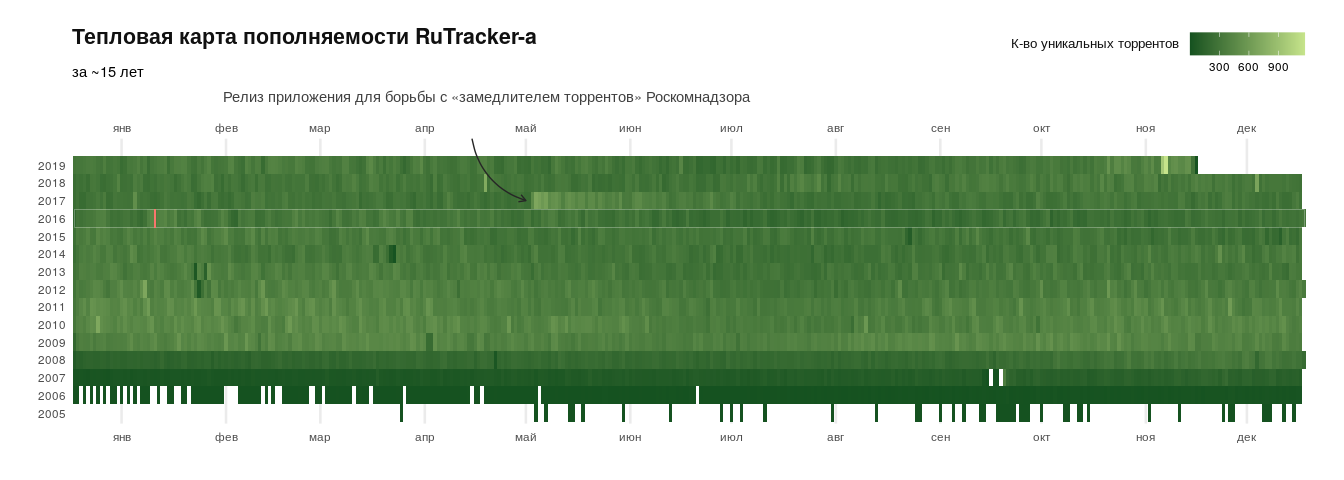
2017 . (. GitHub ). 2016 , . .
. . – .
, content , , , 15 .
Dataiku
, : , , , .
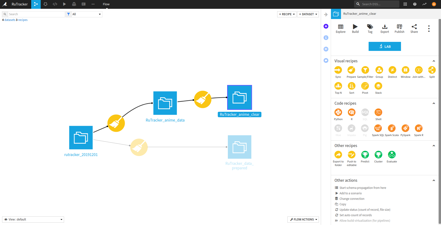
, -. . – .
– .
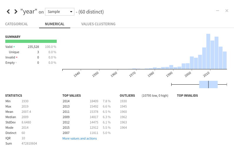
: rutracker.org , , — 60. 2009 — 2014 .
. , , . .
, . .

, dataiku — . , , (R, Python), . .
, RuTracker, : , . . , . .
UPD: , recipe dataiku.
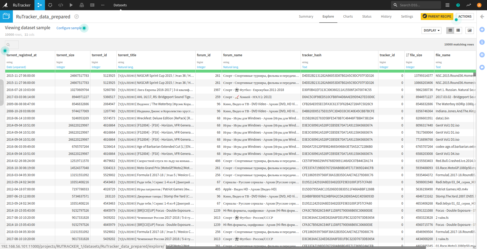
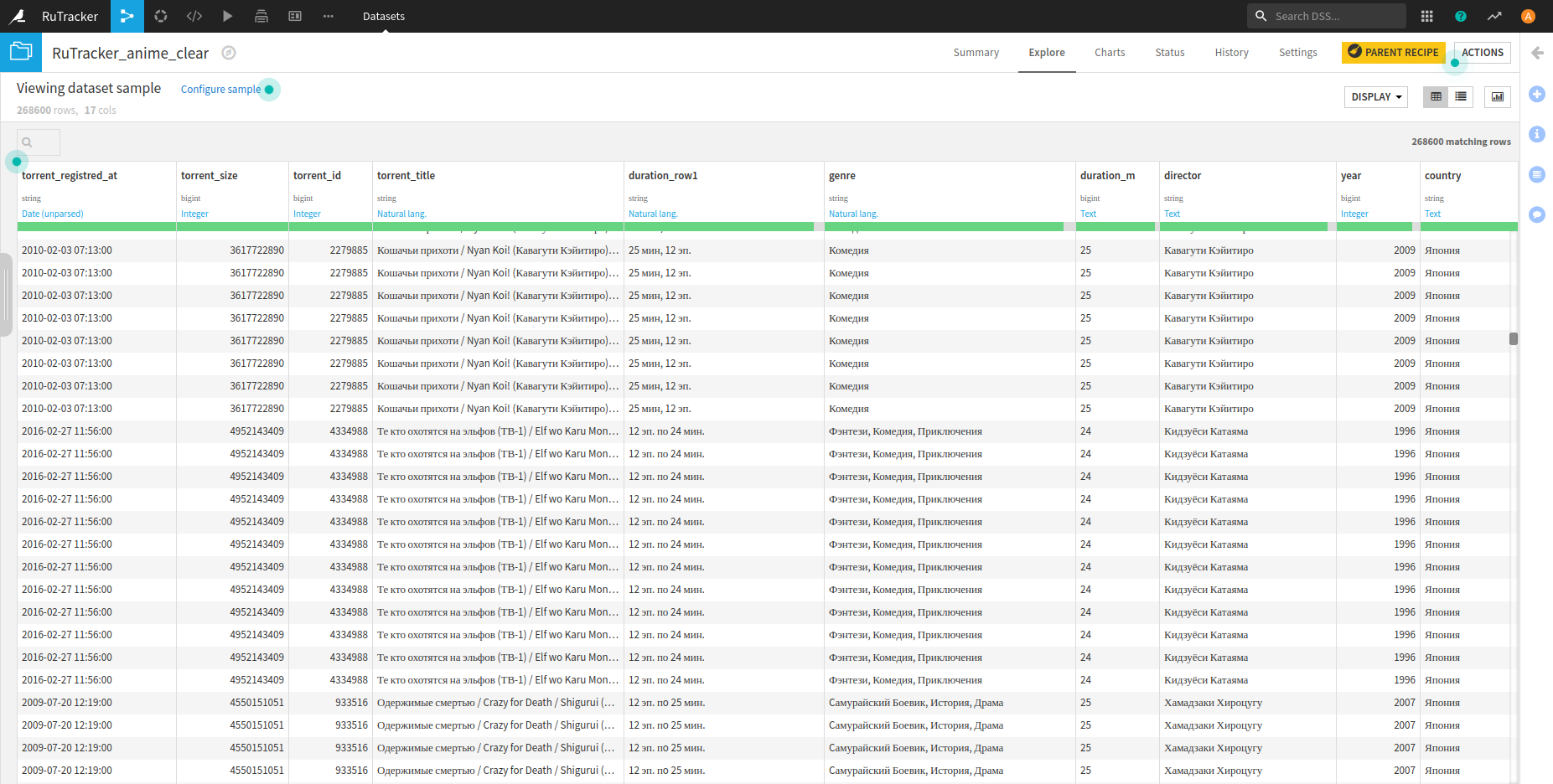
有条件地,本文中给出的方法可以分为两部分:准备要在R中进行分析的数据以及准备要直接在平台上进行分析的有关动漫的数据。
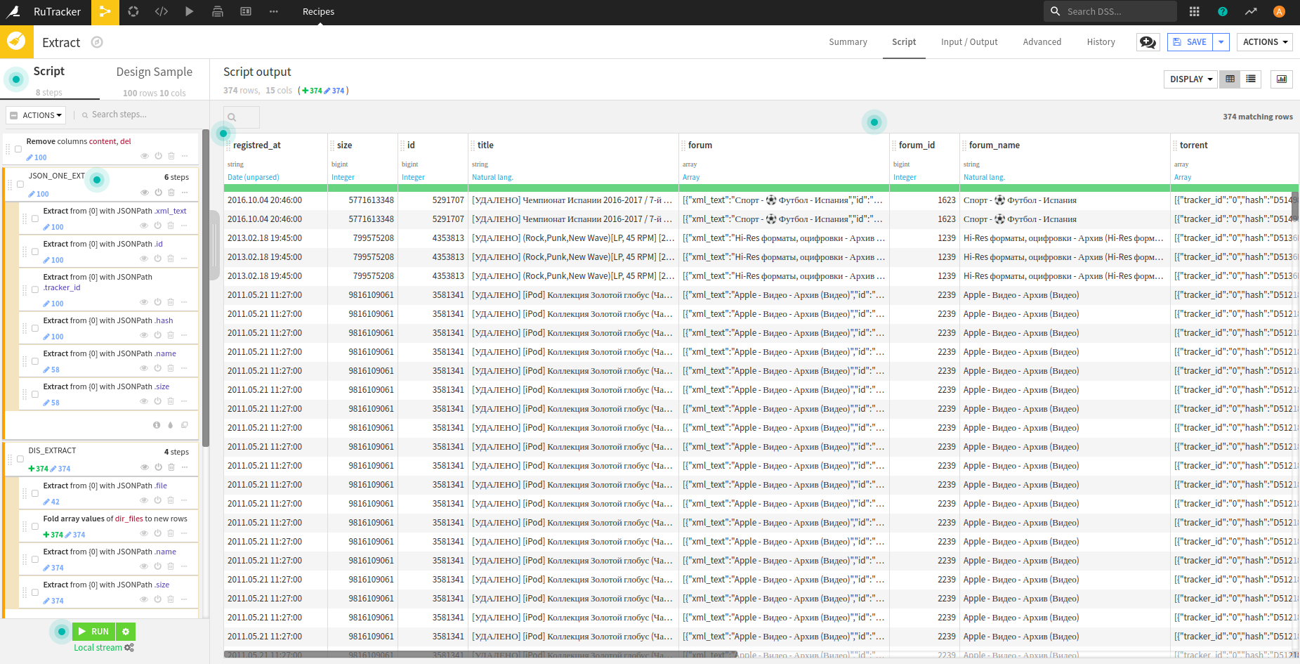
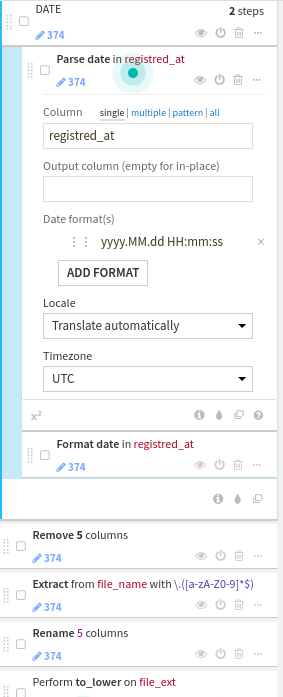
在R中进行分析的准备阶段json- .
json-. .
timestamp .
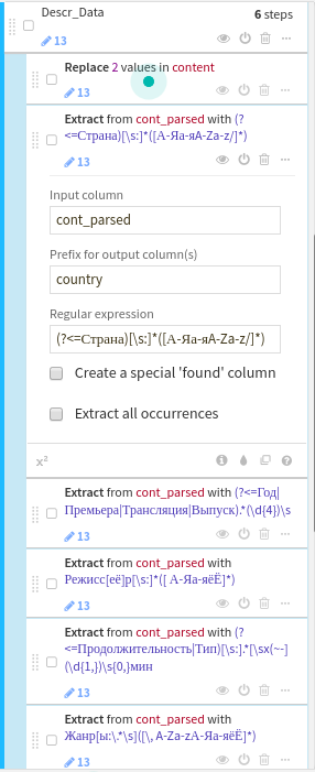
动漫数据准备阶段, , . content — Descr_Data.
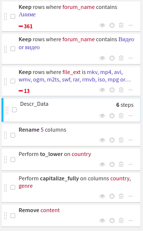
contentregexp , , , . , regexp dataiku .