随机森林，主成分方法和超参数优化：解决Python分类问题的示例

1. 基于RF算法的基本模型（我们将简称为RF模型）。
2. 与1号模型相同，但其中一种模型是使用主成分方法（RF + PCA）来缩小特征空间的尺寸。
3. 与2号模型相同，但使用超参数优化（RF + PCA + HT）构建。

1.导入数据

• df.head() -查看新数据框，看其是否符合预期。
• df.info()-找出数据类型和列内容的特征。在继续之前，可能需要执行数据类型转换。
• df.isna()-确保数据中没有值NaN。相应的值（如果有）可能需要以某种方式处理，或者，如果有必要，可能有必要从数据帧中删除整行。
• df.describe() -找出列中指标的最小，最大值，平均值，找出列中均方根和可能偏差的指标。

import pandas as pd
from sklearn.datasets import load_breast_cancer
columns = ['mean radius', 'mean texture', 'mean perimeter', 'mean area', 'mean smoothness', 'mean compactness', 'mean concavity', 'mean concave points', 'mean symmetry', 'mean fractal dimension', 'radius error', 'texture error', 'perimeter error', 'area error', 'smoothness error', 'compactness error', 'concavity error', 'concave points error', 'symmetry error', 'fractal dimension error', 'worst radius', 'worst texture', 'worst perimeter', 'worst area', 'worst smoothness', 'worst compactness', 'worst concavity', 'worst concave points', 'worst symmetry', 'worst fractal dimension']
dataset = load_breast_cancer()
data = pd.DataFrame(dataset['data'], columns=columns)
data['cancer'] = dataset['target']
display(data.head())
display(data.info())
display(data.isna().sum())
display(data.describe())

2.

from sklearn.model_selection import train_test_split
X = data.drop('cancer', axis=1)  
y = data['cancer'] 
X_train, X_test, y_train, y_test = train_test_split(X, y, test_size=0.50, random_state = 2020, stratify=y)

3.数据缩放

import numpy as np
from sklearn.preprocessing import StandardScaler
ss = StandardScaler()
X_train_scaled = ss.fit_transform(X_train)
X_test_scaled = ss.transform(X_test)
y_train = np.array(y_train)

4.基本模型的训练（RF 1号模型）

from sklearn.ensemble import RandomForestClassifier
from sklearn.metrics import recall_score
rfc = RandomForestClassifier()
rfc.fit(X_train_scaled, y_train)
display(rfc.score(X_train_scaled, y_train))
# 1.0

feats = {}
for feature, importance in zip(data.columns, rfc_1.feature_importances_):
    feats[feature] = importance
importances = pd.DataFrame.from_dict(feats, orient='index').rename(columns={0: 'Gini-Importance'})
importances = importances.sort_values(by='Gini-Importance', ascending=False)
importances = importances.reset_index()
importances = importances.rename(columns={'index': 'Features'})
sns.set(font_scale = 5)
sns.set(style="whitegrid", color_codes=True, font_scale = 1.7)
fig, ax = plt.subplots()
fig.set_size_inches(30,15)
sns.barplot(x=importances['Gini-Importance'], y=importances['Features'], data=importances, color='skyblue')
plt.xlabel('Importance', fontsize=25, weight = 'bold')
plt.ylabel('Features', fontsize=25, weight = 'bold')
plt.title('Feature Importance', fontsize=25, weight = 'bold')
display(plt.show())
display(importances)

5.主成分法

import matplotlib.pyplot as plt
import seaborn as sns
from sklearn.decomposition import PCA
pca_test = PCA(n_components=30)
pca_test.fit(X_train_scaled)
sns.set(style='whitegrid')
plt.plot(np.cumsum(pca_test.explained_variance_ratio_))
plt.xlabel('number of components')
plt.ylabel('cumulative explained variance')
plt.axvline(linewidth=4, color='r', linestyle = '--', x=10, ymin=0, ymax=1)
display(plt.show())
evr = pca_test.explained_variance_ratio_
cvr = np.cumsum(pca_test.explained_variance_ratio_)
pca_df = pd.DataFrame()
pca_df['Cumulative Variance Ratio'] = cvr
pca_df['Explained Variance Ratio'] = evr
display(pca_df.head(10))

pca = PCA(n_components=10)
pca.fit(X_train_scaled)
X_train_scaled_pca = pca.transform(X_train_scaled)
X_test_scaled_pca = pca.transform(X_test_scaled)

pca_dims = []
for x in range(0, len(pca_df)):
    pca_dims.append('PCA Component {}'.format(x))
pca_test_df = pd.DataFrame(pca_test.components_, columns=columns, index=pca_dims)
pca_test_df.head(10).T

6.在对数据应用主成分法之后训练基本的RF模型（模型2，RF + PCA）

rfc = RandomForestClassifier()
rfc.fit(X_train_scaled_pca, y_train)
display(rfc.score(X_train_scaled_pca, y_train))
# 1.0

7.优化超参数。第一轮：RandomizedSearchCV

• n_estimators -“随机森林”中“树”的数量。
• max_features -选择分割的特征数量。
• max_depth -树木的最大深度。
• min_samples_split -树节点分裂所需的最少对象数。
• min_samples_leaf -叶子中的最小对象数。
• bootstrap -用于构造带有返回的子样本树。

from sklearn.model_selection import RandomizedSearchCV
n_estimators = [int(x) for x in np.linspace(start = 100, stop = 1000, num = 10)]
max_features = ['log2', 'sqrt']
max_depth = [int(x) for x in np.linspace(start = 1, stop = 15, num = 15)]
min_samples_split = [int(x) for x in np.linspace(start = 2, stop = 50, num = 10)]
min_samples_leaf = [int(x) for x in np.linspace(start = 2, stop = 50, num = 10)]
bootstrap = [True, False]
param_dist = {'n_estimators': n_estimators,
               'max_features': max_features,
               'max_depth': max_depth,
               'min_samples_split': min_samples_split,
               'min_samples_leaf': min_samples_leaf,
               'bootstrap': bootstrap}
rs = RandomizedSearchCV(rfc_2, 
                        param_dist, 
                        n_iter = 100, 
                        cv = 3, 
                        verbose = 1, 
                        n_jobs=-1, 
                        random_state=0)
rs.fit(X_train_scaled_pca, y_train)
rs.best_params_
# {'n_estimators': 700,
# 'min_samples_split': 2,
# 'min_samples_leaf': 2,
# 'max_features': 'log2',
# 'max_depth': 11,
# 'bootstrap': True}

rs_df = pd.DataFrame(rs.cv_results_).sort_values('rank_test_score').reset_index(drop=True)
rs_df = rs_df.drop([
            'mean_fit_time', 
            'std_fit_time', 
            'mean_score_time',
            'std_score_time', 
            'params', 
            'split0_test_score', 
            'split1_test_score', 
            'split2_test_score', 
            'std_test_score'],
            axis=1)
rs_df.head(10)

fig, axs = plt.subplots(ncols=3, nrows=2)
sns.set(style="whitegrid", color_codes=True, font_scale = 2)
fig.set_size_inches(30,25)
sns.barplot(x='param_n_estimators', y='mean_test_score', data=rs_df, ax=axs[0,0], color='lightgrey')
axs[0,0].set_ylim([.83,.93])axs[0,0].set_title(label = 'n_estimators', size=30, weight='bold')
sns.barplot(x='param_min_samples_split', y='mean_test_score', data=rs_df, ax=axs[0,1], color='coral')
axs[0,1].set_ylim([.85,.93])axs[0,1].set_title(label = 'min_samples_split', size=30, weight='bold')
sns.barplot(x='param_min_samples_leaf', y='mean_test_score', data=rs_df, ax=axs[0,2], color='lightgreen')
axs[0,2].set_ylim([.80,.93])axs[0,2].set_title(label = 'min_samples_leaf', size=30, weight='bold')
sns.barplot(x='param_max_features', y='mean_test_score', data=rs_df, ax=axs[1,0], color='wheat')
axs[1,0].set_ylim([.88,.92])axs[1,0].set_title(label = 'max_features', size=30, weight='bold')
sns.barplot(x='param_max_depth', y='mean_test_score', data=rs_df, ax=axs[1,1], color='lightpink')
axs[1,1].set_ylim([.80,.93])axs[1,1].set_title(label = 'max_depth', size=30, weight='bold')
sns.barplot(x='param_bootstrap',y='mean_test_score', data=rs_df, ax=axs[1,2], color='skyblue')
axs[1,2].set_ylim([.88,.92])
axs[1,2].set_title(label = 'bootstrap', size=30, weight='bold')
plt.show()

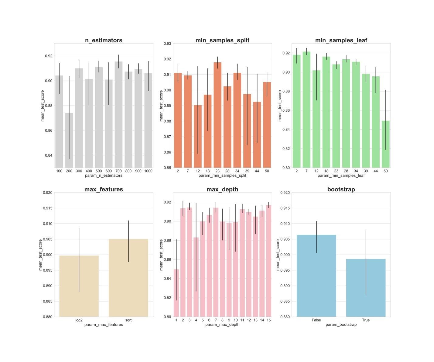
• n_estimators：显然，300、500、700的值显示出最佳的平均结果。
• min_samples_split：像2和7这样的小值似乎显示出最好的结果。值23看起来也不错。您可以检查此超参数超过2的几个值，以及约23的几个值。
• min_samples_leaf：感觉这个超参数的较小值会给出更好的结果。这意味着我们可以体验2到7之间的值。
• max_features：选项sqrt给出最高的平均结果。
• max_depth：超参数的值与模型的结果之间没有明确的关系，但是有一种感觉，值2、3、7、11、15看起来不错。
• bootstrap：该值False显示最佳的平均结果。

8.优化超参数。第2轮：GridSearchCV（模型3的参数的最终准备，RF + PCA + HT）

from sklearn.model_selection import GridSearchCV
n_estimators = [300,500,700]
max_features = ['sqrt']
max_depth = [2,3,7,11,15]
min_samples_split = [2,3,4,22,23,24]
min_samples_leaf = [2,3,4,5,6,7]
bootstrap = [False]
param_grid = {'n_estimators': n_estimators,
               'max_features': max_features,
               'max_depth': max_depth,
               'min_samples_split': min_samples_split,
               'min_samples_leaf': min_samples_leaf,
               'bootstrap': bootstrap}
gs = GridSearchCV(rfc_2, param_grid, cv = 3, verbose = 1, n_jobs=-1)
gs.fit(X_train_scaled_pca, y_train)
rfc_3 = gs.best_estimator_
gs.best_params_
# {'bootstrap': False,
# 'max_depth': 7,
# 'max_features': 'sqrt',
# 'min_samples_leaf': 3,
# 'min_samples_split': 2,
# 'n_estimators': 500}

9.根据验证数据评估模型的质量

y_pred = rfc.predict(X_test_scaled)
y_pred_pca = rfc.predict(X_test_scaled_pca)
y_pred_gs = gs.best_estimator_.predict(X_test_scaled_pca)

from sklearn.metrics import confusion_matrix
conf_matrix_baseline = pd.DataFrame(confusion_matrix(y_test, y_pred), index = ['actual 0', 'actual 1'], columns = ['predicted 0', 'predicted 1'])
conf_matrix_baseline_pca = pd.DataFrame(confusion_matrix(y_test, y_pred_pca), index = ['actual 0', 'actual 1'], columns = ['predicted 0', 'predicted 1'])
conf_matrix_tuned_pca = pd.DataFrame(confusion_matrix(y_test, y_pred_gs), index = ['actual 0', 'actual 1'], columns = ['predicted 0', 'predicted 1'])
display(conf_matrix_baseline)
display('Baseline Random Forest recall score', recall_score(y_test, y_pred))
display(conf_matrix_baseline_pca)
display('Baseline Random Forest With PCA recall score', recall_score(y_test, y_pred_pca))
display(conf_matrix_tuned_pca)
display('Hyperparameter Tuned Random Forest With PCA Reduced Dimensionality recall score', recall_score(y_test, y_pred_gs))

摘要