Qualquer atividade gera dados. Faça o que fizer, provavelmente você tem em suas mãos um depósito de informações úteis brutas ou, pelo menos, acesso à sua fonte.
Hoje, o vencedor é quem toma decisões com base em dados objetivos. As habilidades do analista são mais relevantes do que nunca, e a disponibilidade das ferramentas necessárias disponíveis permite que você esteja sempre um passo à frente. Esta é uma ajuda na aparência deste artigo.
Você tem seu próprio negócio? Ou talvez ... não importa. O processo de mineração de dados é interminável e emocionante. E mesmo cavando bem na Internet, você pode encontrar um campo para atividade.
Aqui está o que temos hoje: um banco de dados de distribuição XML não oficial do RuTracker.ORG. O banco de dados é atualizado a cada seis meses e contém informações sobre todas as distribuições para o histórico da existência desse rastreador de torrents.
O que ela pode dizer aos donos do rutreker? E os cúmplices diretos da pirataria na Internet? Ou um usuário comum que gosta de anime, por exemplo?
Você entende o que eu quero dizer?
Pilha - R, Clickhouse, Dataiku
Qualquer análise passa por vários estágios principais: extração de dados, sua preparação e estudo de dados (visualização). Cada estágio tem sua própria ferramenta. Porque a pilha de hoje:
- R. , Python. dplyr ggplot2. – .
- Clickhouse. . : “clickhouse ” “ ”. , . .
- Dataiku. , -.
: Dataiku . 3 . .
, , , . dataiku .
Big Data – big problems
xml– 5 . – rutracker.org, (2005 .) 2019 . 15 !
R Studio – ! . , .
, R. Big Data, Clickhouse … , xml–. . .
. Dataiku DSS . – 10 000 . . , . , 200 000 .
, . .

. : content — json.
content, . – .
recipe — . , . json .
. , , + dataiku.
recipe, — .
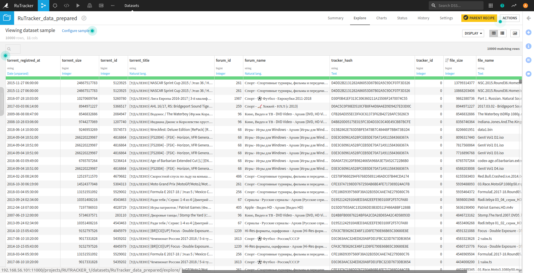
csv Clickhouse.
Clickhouse 15 rutracker-a.
?
SELECT ROUND(uniq(torrent_id) / 1000000, 2) AS Count_M
FROM rutracker

┌─Count_M─┐
│    1.46 │
└─────────┘
1 rows in set. Elapsed: 0.247 sec. Processed 25.51 million rows, 204.06 MB (103.47 million rows/s., 827.77 MB/s.)
1.5 25 . 0.3 ! .
, , .
SELECT COUNT(*) AS Count
FROM rutracker
WHERE (file_ext = 'epub') OR (file_ext = 'fb2') OR (file_ext = 'mobi')

┌──Count─┐
│ 333654 │
└────────┘
1 rows in set. Elapsed: 0.435 sec. Processed 25.51 million rows, 308.79 MB (58.64 million rows/s., 709.86 MB/s.)
300 — ! , . .
SELECT ROUND(SUM(file_size) / 1000000000, 2) AS Total_size_GB
FROM rutracker
WHERE (file_ext = 'epub') OR (file_ext = 'fb2') OR (file_ext = 'mobi')

┌─Total_size_GB─┐
│        625.75 │
└───────────────┘
1 rows in set. Elapsed: 0.296 sec. Processed 25.51 million rows, 344.32 MB (86.24 million rows/s., 1.16 GB/s.)
– 25 . , ?
R
R. , DBI ( ). Clickhouse.
Rlibrary(DBI) # , ... Clickhouse
library(dplyr) # %>%
#
library(ggplot2)
library(ggrepel)
library(cowplot)
library(scales)
library(ggrepel)
# localhost:9000
connection <- dbConnect(RClickhouse::clickhouse(), host="localhost", port = 9000)
, . dplyr .
? rutracker.org .
Ryears_stat <- dbGetQuery(connection,
"SELECT
round(COUNT(*)/1000000, 2) AS Files,
round(uniq(torrent_id)/1000, 2) AS Torrents,
toYear(torrent_registred_at) AS Year
FROM rutracker
GROUP BY Year")
ggplot(years_stat, aes(as.factor(Year), as.double(Files))) +
geom_bar(stat = 'identity', fill = "darkblue", alpha = 0.8)+
theme_minimal() +
labs(title = " RuTracker", subtitle = " 2005 - 2019\n")+
theme(axis.text.x = element_text(angle=90, vjust = 0.5),
axis.text.y = element_text(),
axis.title.y = element_blank(),
axis.title.x = element_blank(),
panel.grid.major.x = element_blank(),
panel.grid.major.y = element_line(size = 0.9),
panel.grid.minor.y = element_line(size = 0.4),
plot.title = element_text(vjust = 3, hjust = 0, family = "sans", size = 16, color = "#101010", face = "bold"),
plot.caption = element_text(vjust = 3, hjust = 0, family = "sans", size = 12, color = "#101010", face = "bold"),
plot.margin = unit(c(1,0.5,1,0.5), "cm"))+
scale_y_continuous(labels = number_format(accuracy = 1, suffix = " "))
ggplot(years_stat, aes(as.factor(Year), as.integer(Torrents))) +
geom_bar(stat = 'identity', fill = "#008b8b", alpha = 0.8)+
theme_minimal() +
labs(title = " RuTracker", subtitle = " 2005 - 2019\n", caption = "* ")+
theme(axis.text.x = element_text(angle=90, vjust = 0.5),
axis.text.y = element_text(),
axis.title.y = element_blank(),
axis.title.x = element_blank(),
panel.grid.major.x = element_blank(),
panel.grid.major.y = element_line(size = 0.9),
panel.grid.minor.y = element_line(size = 0.4),
plot.title = element_text(vjust = 3, hjust = 0, family = "sans", size = 16, color = "#101010", face = "bold"),
plot.caption = element_text(vjust = -3, hjust = 1, family = "sans", size = 9, color = "grey60", face = "plain"),
plot.margin = unit(c(1,0.5,1,0.5), "cm")) +
scale_y_continuous(labels = number_format(accuracy = 1, suffix = " "))
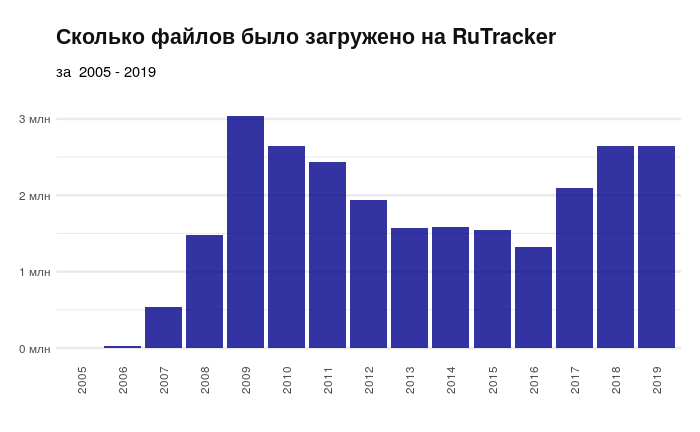
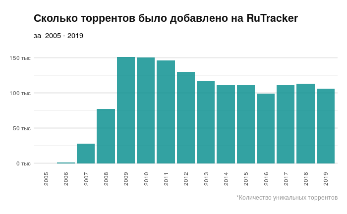
2016 . , 2016 rutracker.org . , .
, . , .
.
Rextention_stat <- dbGetQuery(connection,
"SELECT toYear(torrent_registred_at) AS Year,
COUNT(tracker_id)/1000 AS Count,
ROUND(SUM(file_size)/1000000000000, 2) AS Total_Size_TB,
file_ext
FROM rutracker
GROUP BY Year, file_ext
ORDER BY Year, Count")
#
TopExt <- function(x, n) {
res_tab <- NULL
# 2005 2006, ..
for (i in (3:15)) {
res_tab <-bind_rows(list(res_tab,
extention_stat %>% filter(Year == x[i]) %>%
arrange(desc(Count), desc(Total_Size_TB)) %>%
head(n)
))
}
return(res_tab)
}
years_list <- unique(extention_stat$Year)
ext_data <- TopExt(years_list, 5)
ggplot(ext_data, aes(as.factor(Year), as.integer(Count), fill = file_ext)) +
geom_bar(stat = "identity",position="dodge2", alpha =0.8, width = 1)+
theme_minimal() +
labs(title = " RuTracker",
subtitle = " 2005 - 2019\n",
caption = "* -5 ", fill = "") +
theme(axis.text.x = element_text(angle=90, vjust = 0.5),
axis.text.y = element_text(),
axis.title.y = element_blank(),
axis.title.x = element_blank(),
panel.grid.major.x = element_blank(),
panel.grid.major.y = element_line(size = 0.9),
panel.grid.minor.y = element_line(size = 0.4),
legend.title = element_text(vjust = 1, hjust = -1, family = "sans", size = 9, color = "#101010", face = "plain"),
legend.position = "top",
plot.title = element_text(vjust = 3, hjust = 0, family = "sans", size = 16, color = "#101010", face = "bold"),
plot.caption = element_text(vjust = -4, hjust = 1, family = "sans", size = 9, color = "grey60", face = "plain"),
plot.margin = unit(c(1,0.5,1,0.5), "cm")) +
scale_y_continuous(labels = number_format(accuracy = 0.5, scale = (1/1000), suffix = " "))+guides(fill=guide_legend(nrow=1))
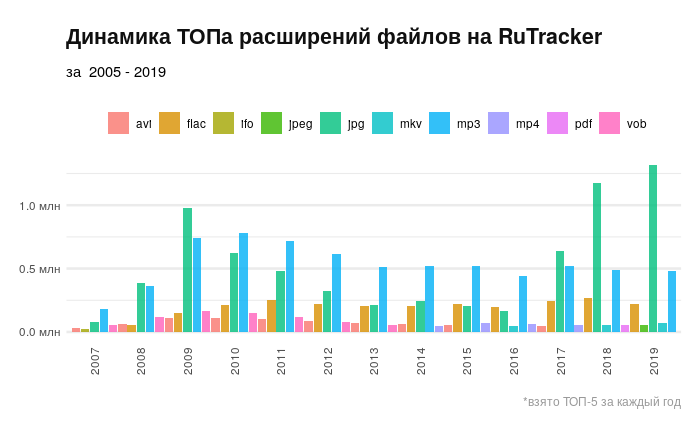
. . .
rutracker-a. .
Rchapter_stat <- dbGetQuery(connection,
"SELECT
substring(forum_name, 1, position(forum_name, ' -')) Chapter,
uniq(torrent_id) AS Count,
ROUND(median(file_size)/1000000, 2) AS Median_Size_MB,
ROUND(max(file_size)/1000000000) AS Max_Size_GB,
ROUND(SUM(file_size)/1000000000000) AS Total_Size_TB
FROM rutracker WHERE Chapter NOT LIKE('\"%')
GROUP BY Chapter
ORDER BY Count DESC")
chapter_stat$Count <- as.integer(chapter_stat$Count)
#
AggChapter2 <- function(Chapter){
var_ch <- str(Chapter)
res = NULL
for(i in (1:22)){
select_str <-paste0(
"SELECT
toYear(torrent_registred_at) AS Year,
substring(forum_name, 1, position(forum_name, ' -')) Chapter,
uniq(torrent_id)/1000 AS Count,
ROUND(median(file_size)/1000000, 2) AS Median_Size_MB,
ROUND(max(file_size)/1000000000,2) AS Max_Size_GB,
ROUND(SUM(file_size)/1000000000000,2) AS Total_Size_TB
FROM rutracker
WHERE Chapter LIKE('", Chapter[i], "%')
GROUP BY Year, Chapter
ORDER BY Year")
res <-bind_rows(list(res, dbGetQuery(connection, select_str)))
}
return(res)
}
chapters_data <- AggChapter2(chapter_stat$Chapter)
chapters_data$Chapter <- as.factor(chapters_data$Chapter)
chapters_data$Count <- as.numeric(chapters_data$Count)
chapters_data %>% group_by(Chapter)%>%
ggplot(mapping = aes(x = reorder(Chapter, Total_Size_TB), y = Total_Size_TB))+
geom_bar(stat = "identity", fill="darkblue", alpha =0.8)+
theme(panel.grid.major.x = element_line(colour="grey60", linetype="dashed"))+
xlab('\n') + theme_minimal() +
labs(title = "C RuTracker-",
subtitle = " 2019\n")+
theme(axis.text.x = element_text(),
axis.text.y = element_text(family = "sans", size = 9, color = "#101010", hjust = 1, vjust = 0.5),
axis.title.y = element_text(vjust = 2.5, hjust = 0, family = "sans", size = 9, color = "grey40", face = "plain"),
axis.title.x = element_blank(),
axis.line.x = element_line(color = "grey60", size = 0.1, linetype = "solid"),
panel.grid.major.y = element_blank(),
panel.grid.major.x = element_line(size = 0.7, linetype = "solid"),
panel.grid.minor.x = element_line(size = 0.4, linetype = "solid"),
plot.title = element_text(vjust = 3, hjust = 1, family = "sans", size = 16, color = "#101010", face = "bold"),
plot.subtitle = element_text(vjust = 2, hjust = 1, family = "sans", size = 12, color = "#101010", face = "plain"),
plot.caption = element_text(vjust = -3, hjust = 1, family = "sans", size = 9, color = "grey60", face = "plain"),
plot.margin = unit(c(1,0.5,1,0.5), "cm"))+
scale_y_continuous(labels = number_format(accuracy = 1, suffix = " "))+
coord_flip()
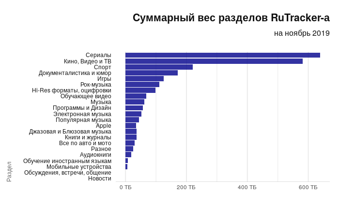
. — — . , . , Apple.
Rchapters_data %>% group_by(Chapter)%>%
ggplot(mapping = aes(x = reorder(Chapter, Count), y = Count))+
geom_bar(stat = "identity", fill="#008b8b", alpha =0.8)+
theme(panel.grid.major.x = element_line(colour="grey60", linetype="dashed"))+
xlab('') + theme_minimal() +
labs(title = " RuTracker-",
subtitle = " 2019\n")+
theme(axis.text.x = element_text(),
axis.text.y = element_text(family = "sans", size = 9, color = "#101010", hjust = 1, vjust = 0.5),
axis.title.y = element_text(vjust = 3.5, hjust = 0, family = "sans", size = 9, color = "grey40", face = "plain"),
axis.title.x = element_blank(),
axis.line.x = element_line(color = "grey60", size = 0.1, linetype = "solid"),
panel.grid.major.y = element_blank(),
panel.grid.major.x = element_line(size = 0.7, linetype = "solid"),
panel.grid.minor.x = element_line(size = 0.4, linetype = "solid"),
plot.title = element_text(vjust = 3, hjust = 1, family = "sans", size = 16, color = "#101010", face = "bold"),
plot.subtitle = element_text(vjust = 2, hjust = 1, family = "sans", size = 12, color = "#101010", face = "plain"),
plot.caption = element_text(vjust = -3, hjust = 1, family = "sans", size = 9, color = "grey60", face = "plain"),
plot.margin = unit(c(1,0.5,1,0.5), "cm"))+
scale_y_continuous(limits = c(0, 300), labels = number_format(accuracy = 1, suffix = " "))+
coord_flip()
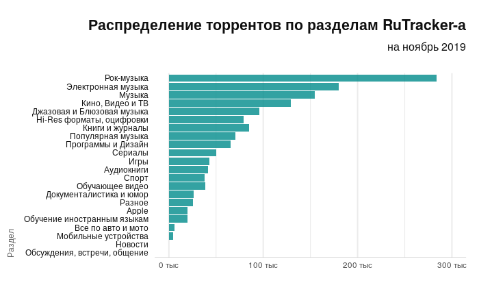
, , : -.
~15 .
Rlibrary("RColorBrewer")
getPalette = colorRampPalette(brewer.pal(19, "Spectral"))
chapters_data %>% #filter(Chapter %in% chapter_stat$Chapter[c(4,6,7,9:20)])%>%
filter(!Chapter %in% chapter_stat$Chapter[c(16, 21, 22)])%>%
filter(Year>=2007)%>%
ggplot(mapping = aes(x = Year, y = Count, fill = as.factor(Chapter)))+
geom_area(alpha =0.8, position = "fill")+
theme_minimal() +
labs(title = " -",
subtitle = " ~15 ", fill = "")+
theme(axis.text.x = element_text(vjust = 0.5),
axis.text.y = element_blank(),
axis.title.y = element_blank(),
axis.title.x = element_blank(),
panel.grid.major.x = element_blank(),
panel.grid.major.y = element_line(size = 0.9),
panel.grid.minor.y = element_line(size = 0.4),
plot.title = element_text(vjust = 3, hjust = 0, family = "sans", size = 16, color = "#101010", face = "bold"),
plot.caption = element_text(vjust = -3, hjust = 1, family = "sans", size = 9, color = "grey60", face = "plain"),
plot.margin = unit(c(1,1,1,1), "cm")) +
scale_x_continuous(breaks = c(2008, 2010, 2012, 2014, 2016, 2018),expand=c(0,0)) +
scale_fill_manual(values = getPalette(19))
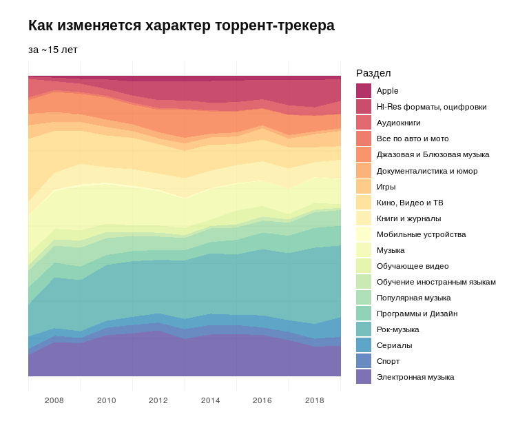
- — . — Apple , .
. .
, Rutracker-a. - rutracker.org.
Runique_torr_per_day <- dbGetQuery(connection,
"SELECT toDate(torrent_registred_at) AS date,
uniq(torrent_id) AS count
FROM rutracker
GROUP BY date
ORDER BY date")
unique_torr_per_day %>%
ggplot(aes(format(date, "%Y"), format(date, "%j"), fill = as.numeric(count)))+
geom_tile() +
theme_minimal() +
labs(title = " RuTracker-a",
subtitle = " ~15 \n\n",
fill = "- \n")+
theme(axis.text.x = element_text(vjust = 0.5),
axis.text.y = element_text(),
axis.title.y = element_blank(),
axis.title.x = element_blank(),
panel.grid.major.y = element_blank(),
panel.grid.major.x = element_line(size = 0.9),
panel.grid.minor.x = element_line(size = 0.4),
legend.title = element_text(vjust = 0.7, hjust = -1, family = "sans", size = 10, color = "#101010", face = "plain"),
legend.position = c(0.88, 1.30),
legend.direction = "horizontal",
plot.title = element_text(vjust = 3, hjust = 0, family = "sans", size = 16, color = "#101010", face = "bold"),
plot.caption = element_text(vjust = -3, hjust = 1, family = "sans", size = 9, color = "grey60", face = "plain"),
plot.margin = unit(c(1,1,1,1), "cm"))+ coord_flip(clip = "off") +
scale_y_discrete(breaks = c(format(as.Date("2007-01-15"), "%j"),
format(as.Date("2007-02-15"), "%j"),
format(as.Date("2007-03-15"), "%j"),
format(as.Date("2007-04-15"), "%j"),
format(as.Date("2007-05-15"), "%j"),
format(as.Date("2007-06-15"), "%j"),
format(as.Date("2007-07-15"), "%j"),
format(as.Date("2007-08-15"), "%j"),
format(as.Date("2007-09-15"), "%j"),
format(as.Date("2007-10-15"), "%j"),
format(as.Date("2007-11-15"), "%j"),
format(as.Date("2007-12-15"), "%j")),
labels = c("", "", "", "", "", "","", "", "", "","",""), position = 'right') +
scale_fill_gradientn(colours = c("#155220", "#c6e48b")) +
annotate(geom = "curve", x = 16.5, y = 119, xend = 13, yend = 135,
curvature = .3, color = "grey15", arrow = arrow(length = unit(2, "mm"))) +
annotate(geom = "text", x = 16, y = 45,
label = " « » \n",
hjust = "left", vjust = -0.75, color = "grey25") +
guides(x.sec = guide_axis_label_trans(~.x)) +
annotate("rect", xmin = 11.5, xmax = 12.5, ymin = 1, ymax = 366,
alpha = .0, colour = "white", size = 0.1) +
geom_segment(aes(x = 11.5, y = 25, xend = 12.5, yend = 25, colour = "segment"),
show.legend = FALSE)
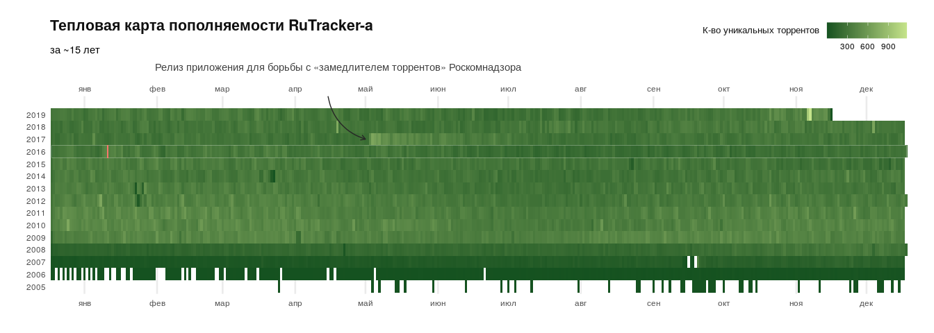
2017 . (. GitHub ). 2016 , . .
. . – .
, content , , , 15 .
Dataiku
, : , , , .
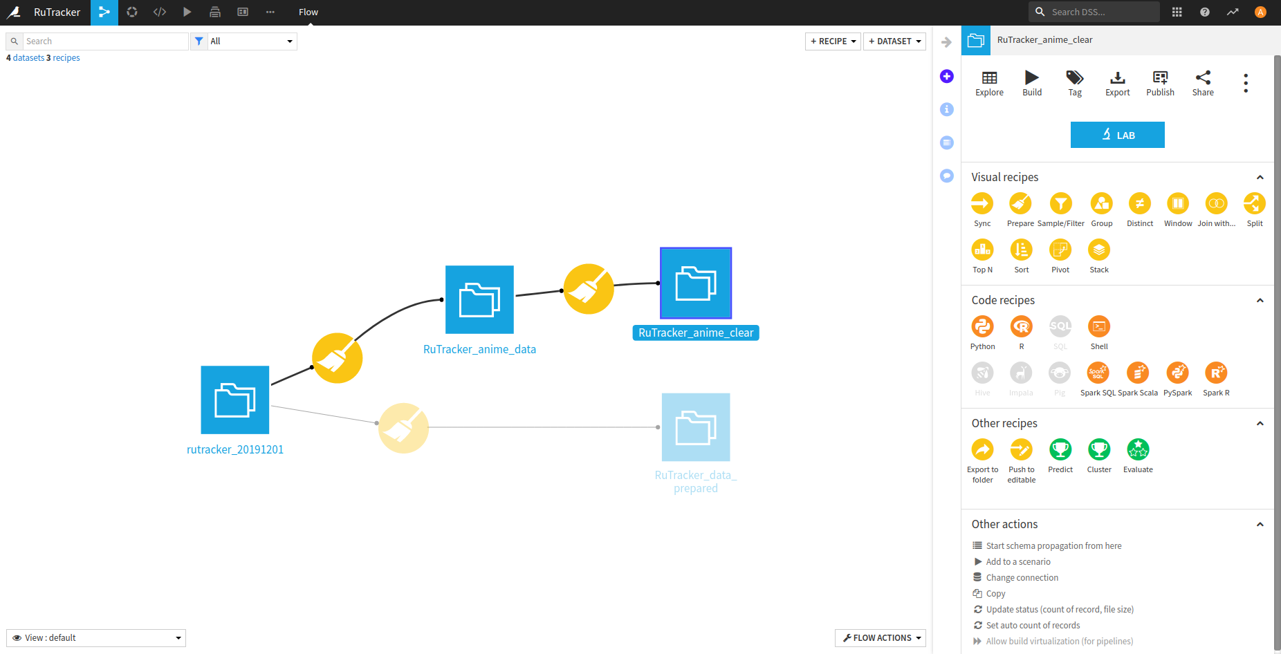
, -. . – .
– .
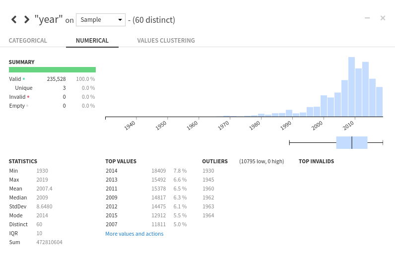
: rutracker.org , , — 60. 2009 — 2014 .
. , , . .
, . .

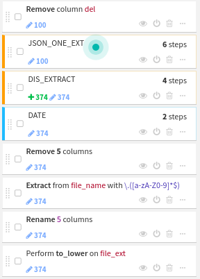
, dataiku — . , , (R, Python), . .
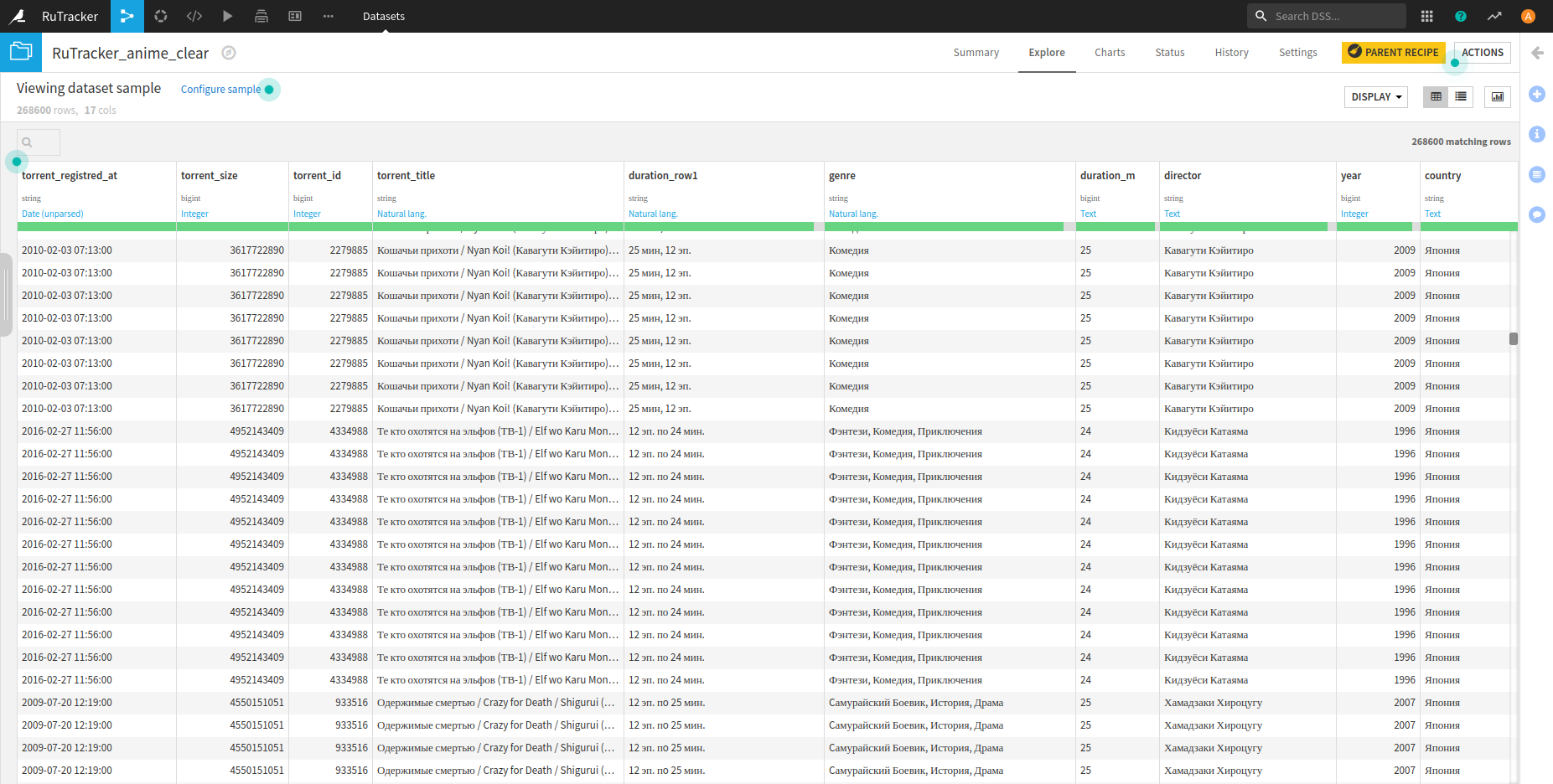
, RuTracker, : , . . , . .
UPD: , recipe dataiku.
Condicionalmente, a receita apresentada neste artigo pode ser dividida em duas partes: preparando dados para análise em R e preparando dados sobre anime para análise diretamente na plataforma.
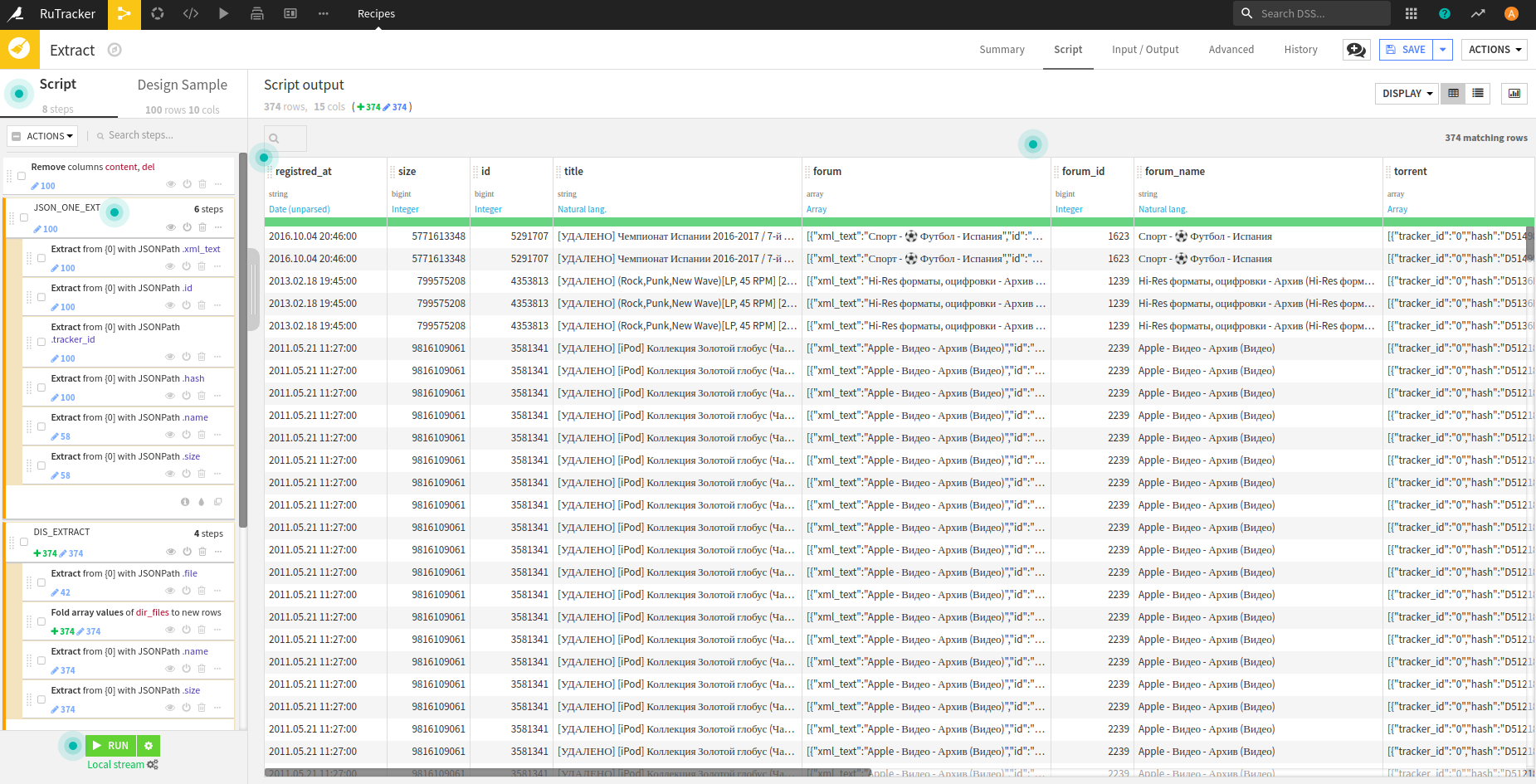
Estágio de preparação para análise em Rjson- .
json-. .
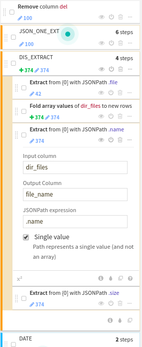
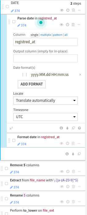
timestamp .
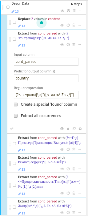
Fase de preparação dos dados do anime, , . content — Descr_Data.
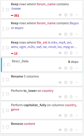
contentregexp , , , . , regexp dataiku .