Pada 13 Maret, di saluran resmi Eurovision YouTube, komposisi grup Little Big telah diposting, yang akan mewakili Rusia di kompetisi. Setelah menonton klipnya, saya ingin membandingkan statistik video grup kami dengan video peserta lainnya; video mana yang paling banyak ditonton, yang memiliki persentase suka tertinggi, yang paling sering dikomentari. Googling statistik yang sudah selesai tidak mengarah ke apa pun. Oleh karena itu, diputuskan untuk mengumpulkan statistik yang diperlukan.
Struktur artikel:
Membuka daftar putar peserta, Anda dapat melihat 39 video, bahkan ada 38 lagu, komposisi Hurricane - Hasta La Vista - Serbia diunduh dua kali, sehingga statistik di dalamnya akan disimpulkan. Untuk mengumpulkan statistik, kami akan menggunakan R.
Kode Unggah
Kami akan membutuhkan paket-paket berikut:
library(tuber) #    API YouTube,
library(dplyr) #
library(ggplot2) #
Pertama, buka konsol pengembang google dan buat kunci OAuth di api API Data YouTube v3. Setelah menerima kunci, login dari R.
yt_oauth(" ", " ")
Sekarang kita dapat mengumpulkan statistik:
#
list_videos <- get_playlist_items(filter = c(playlist_id = "PLmWYEDTNOGUL69D2wj9m2onBKV2s3uT5Y"))

#    ,  get_stats
stats_videos <- lapply(as.character(list_videos$contentDetails.videoId), get_stats) %>%
  bind_rows()
stats_videos <- stats_videos %>%
  mutate_at(vars(-id), as.integer)

#   ,  get_video_details
description_videos <- lapply(as.character(list_videos$contentDetails.videoId), get_video_details)
description_videos <- lapply(description_videos, function(x) {
    list(
      id = x[["items"]][[1]][["id"]],
      name_video = x[["items"]][[1]][["snippet"]][["title"]]
    )
  }) %>%
  bind_rows()
.. — — [ ] — Official Music Video — Eurovision 2020, , . .
#
description_videos$name_video <- description_videos$name_video %>%
  gsub("[^[:alnum:][:blank:]?&/\\-]", '', .) %>%
  gsub("(  .*)|( - Offic.*)", '', .)

#
df <- description_videos %>%
  left_join(stats_videos, by = 'id') %>%
  rowwise() %>%
  mutate( #
    proc_like = round(likeCount / (likeCount + dislikeCount), 2)
    ) %>%
  ungroup()

# Hurricane - Hasta La Vista - Serbia     ,
df <- df %>%
  group_by(name_video) %>%
  summarise(
    id = first(id),
    viewCount = sum(viewCount),
    likeCount = sum(likeCount),
    dislikeCount = sum(dislikeCount),
    commentCount = sum(commentCount),
    proc_like = round(likeCount / (likeCount + dislikeCount), 2)
  )

df$color <- ifelse(df$name_video == 'Little Big - Uno - Russia','red','gray')
. .
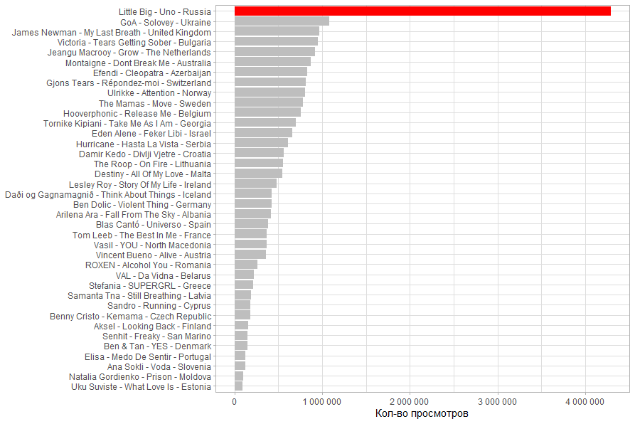
# -
ggplot(df, aes(x = reorder(name_video, viewCount), y = viewCount, fill = color)) +
geom_col() +
coord_flip() +
theme_light() +
labs(x = NULL, y = "- ") +
guides(fill = F) +
scale_fill_manual(values = c('gray', 'red')) +
scale_y_continuous(labels = scales::number_format(big.mark = " "))
#
ggplot(df, aes(x = reorder(name_video, proc_like), y = proc_like, fill = color)) +
geom_col() +
coord_flip() +
theme_light() +
labs(x = NULL, y = " ") +
guides(fill = F) +
scale_fill_manual(values = c('gray', 'red')) +
scale_y_continuous(labels = scales::percent_format(accuracy = 1))
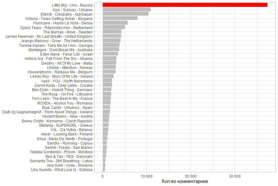
# -
ggplot(df, aes(x = reorder(name_video, commentCount), y = commentCount, fill = color)) +
geom_col() +
coord_flip() +
theme_light() +
labs(x = NULL, y = "- ") +
guides(fill = F) +
scale_fill_manual(values = c('gray', 'red')) +
scale_y_continuous(labels = scales::number_format(big.mark = " "))
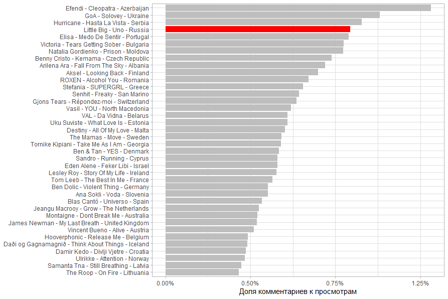
#
ggplot(df, aes(x = reorder(name_video, commentCount/viewCount), y = commentCount/viewCount, fill = color)) +
geom_col() +
coord_flip() +
theme_light() +
labs(x = NULL, y = " ") +
guides(fill = F) +
scale_fill_manual(values = c('gray', 'red')) +
scale_y_continuous(labels = scales::percent_format(accuracy = 0.25))
, Little Big 1 , .
. Little Big , . - .
, . . .

.
( / ). . .
13.03.2020 18:00 , , , .
UPD: 14.03.2020 20:30
. . Little Big , .

, . Little Big ,

.

( / ). 2 , , , . .

14.03.2020 20:30 , , , , . .
:
helg1978 . .
library(rvest)
library(tidyr)

#
hdoc <- read_html('https://en.wikipedia.org/wiki/List_of_countries_and_dependencies_by_population')

tnode <- html_node(hdoc, xpath = '/html/body/div[3]/div[3]/div[4]/div/table')
df_population <- html_table(tnode)

df_population <- df_population %>% filter(`Country (or dependent territory)` != 'World')

df_population$Population <- as.integer(gsub(',','',df_population$Population,fixed = T))

df_population$`Country (or dependent territory)` <- gsub('\\[.*\\]','', df_population$`Country (or dependent territory)`)

df_population <- df_population %>%
  select(
    `Country (or dependent territory)`,
    Population
    ) %>%
  rename(Country = `Country (or dependent territory)`)

#
df2 <- df %>%
  separate(name_video, c('compozitor', 'name_track', 'Country'), ' - ', remove = F) %>%
  mutate(Country = ifelse(Country == 'The Netherlands', 'Netherlands', Country)) %>%
  left_join(df_population, by = 'Country')

#
cor(df2$viewCount,df2$Population)
ggplot(df2, aes(x = Population, y =  viewCount)) +
  geom_point() +
  theme_light() +
  geom_smooth(method = 'lm') +
  labs(x = ", ", y = "- ") +
  scale_y_continuous(labels = scales::number_format(big.mark = " ")) +
  scale_x_continuous(labels = scales::number_format(big.mark = " "))

#     ,
cor(df2[df2$Country != 'Russia',]$viewCount,df2[df2$Country != 'Russia',]$Population)
ggplot(df2 %>% filter(Country != 'Russia') , aes(x = Population, y = viewCount)) +
  geom_point() +
  theme_light() +
  geom_smooth(method = 'lm') +
  labs(x = ", ", y = "- ") +
  scale_y_continuous(labels = scales::number_format(big.mark = " ")) +
  scale_x_continuous(labels = scales::number_format(big.mark = " "))

#     ,
cor(df2$viewCount,df2$Population, method = "spearman")
ggplot(df2 , aes(x = rank(Population), y = rank(viewCount))) +
  geom_point() +
  theme_light() +
  geom_smooth(method = 'lm') +
  labs(x = ",  (  1  40)", y = "-  (  1  40)") +
  guides(fill = F)

#
ggplot(df2, aes(x = reorder(name_video, viewCount/Population), y = viewCount/Population, fill = color)) +
  geom_col() +
  coord_flip() +
  theme_light() +
  labs(x = NULL, y = "    ") +
  guides(fill = F) +
  scale_fill_manual(values = c('gray', 'red')) +
  scale_y_continuous(labels = scales::percent_format(accuracy = 0.25))
, , 50 . 71%.

. 71% 15%. .

( ), , (. . 40%).

Dan sebagai referensi saya menghitung pangsa pandangan dari populasi negara itu. Untuk negara-negara kecil khususnya, ternyata mereka lebih banyak ditonton dari negara lain. Secara khusus, itu adalah Malta, San Marino dan Islandia.

Kode github lengkap