La classification des documents ou du texte est l'une des tâches les plus importantes du traitement du langage naturel (PNL).

Il a de nombreuses utilisations, telles que la catégorisation des nouvelles, le filtrage du spam, la recherche de commentaires inappropriés, etc.

Les grandes entreprises n'ont aucun problème à collecter de grands ensembles de données, donc l'apprentissage d'un modèle de classification de texte à partir de zéro est une tâche réalisable.

Cependant, pour la plupart des tâches du monde réel, les ensembles de données volumineux sont rares et vous devez être intelligent pour créer votre modèle.

Dans cet article, je parlerai d'approches pratiques aux transformations de texte qui permettront de classer les documents, même si l'ensemble de données est petit.

Introduction à la classification des documents

Le processus de classification des documents commence par le nettoyage et la préparation du corps.
Ensuite, ce corps est codé avec n'importe quel type de représentation de texte, après quoi vous pouvez commencer la modélisation.

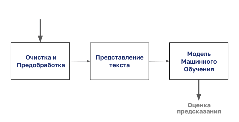
Dans cet article, nous nous concentrerons sur l'étape «Présentation du texte» de ce diagramme.

Ensemble de données de test pour la classification

Nous utiliserons les données du concours. Vrai ou pas? PNL avec les tweets de catastrophe de Kaggle .

Le défi consiste à prédire quels tweets concernaient de véritables catastrophes et lesquels ne l'étaient pas.

Si vous souhaitez répéter l'article étape par étape, n'oubliez pas d'installer les bibliothèques qui y sont utilisées.

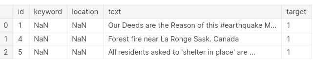
import pandas as pd

tweet= pd.read_csv('../input/nlp-getting-started/train.csv')
test=pd.read_csv('../input/nlp-getting-started/test.csv')

tweet.head(3)

, , , .

print('There are {} rows and {} columns in train'.format(tweet.shape[0],tweet.shape[1]))
print('There are {} rows and {} columns in test'.format(test.shape[0],test.shape[1]))

8000 .

, 280 .

, NLP, .

, , , .

, :

— .
- — «a» «the».
— («studies», «studing» → «study»).

def preprocess_news(df):
    '''Function to preprocess and create corpus'''
    new_corpus=[]

    lem=WordNetLemmatizer()
    for text in df["question_text"]:
        words=[w for w in word_tokenize(text) if (w not in stop)]

        words=[lem.lemmatize(w) for w in words]

        new_corpus.append(words)
    return new_corpus

corpus=preprocess_news(df)

, , .

, .

CountVectorizer

CountVectorizer — .

, , .

text = ["She sells seashells in the seashore"]
# create the transform
vectorizer = CountVectorizer()
# tokenize and build vocab
vectorizer.fit(text)
# summarize
print(vectorizer.vocabulary_)
# encode document
vector = vectorizer.transform(text)
# summarize encoded vector
print(vector.shape)
print(type(vector))
print(vector.toarray())

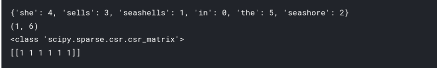
, CountVectorizer Numpy, .

, , .

vector=vectorizer.transform(["I sell seashells in the seashore"])
vector.toarray()

, :

3 4 , . , .

, — «sells» «she».

CountVectorizer, .

vec=CountVectorizer(max_df=10,max_features=10000)
vec.fit(df.question_text.values)
vector=vec.transform(df.question_text.values)

, CountVectorizer , :

max_features — n , .
min_df — , .
max_df — , .

( ).

TfidfVectorizer

Countvectorizer , , "the" ( ) .

— TfidfVectorizer.

— Term frequency-inverse document frequency ( — ).

(Term Frequency) — , .
(Inverse Document Frequency) — , .

from sklearn.feature_extraction.text import TfidfVectorizer
# list of text documents
text = ["She sells seashells by the seashore","The sea.","The seashore"]
# create the transform
vectorizer = TfidfVectorizer()
# tokenize and build vocab
vectorizer.fit(text)
# summarize
print(vectorizer.vocabulary_)
print(vectorizer.idf_)
# encode document
vector = vectorizer.transform([text[0]])
# summarize encoded vector
print(vector.shape)
print(vector.toarray())

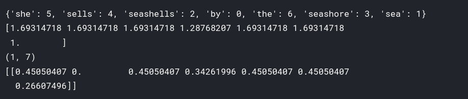
6 , «the», 4 .

0 1, - .

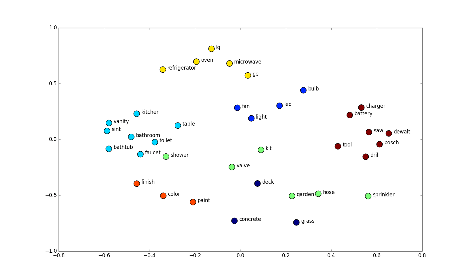
Word2vec

, .

(embeddings) .

n- .

Word2Vec Google .

, .

, , .

«The cat sat on the mat».

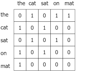
Word2vec :

(Continuous Bag of Words, CBoW) — , .
Skip-Gram — .

, , , . word2vec python:

import gensim
from gensim.models import Word2Vec

model = gensim.models.Word2Vec(corpus, 
                               min_count = 1, size = 100, window = 5)

, word2vec.

size — .
min_count — .
window — , . .

, gensim.

from  gensim.models.KeyedVectors import load_word2vec_format

def load_word2vec():
    word2vecDict = load_word2vec_format(
        '../input/word2vec-google/GoogleNews-vectors-negative300.bin',
        binary=True, unicode_errors='ignore')
    embeddings_index = dict()
    for word in word2vecDict.wv.vocab:
        embeddings_index[word] = word2vecDict.word_vec(word)

    return embeddings_index

w2v_model=load_word2vec()
w2v_model['London'].shape

, 300- .

( — , . , , . . )
, .

FastText

Genism — FastText.

Facebook .

Continuous Bag of Words Skip-Gram.
FastText , n-.

, , «orange».

«ora», «ran», «ang», «nge» ( ).

( ) «orange» n-.

, n- .

, «stupedofantabulouslyfantastic», , , , genism , .

FastText , , .

«fantastic» «fantabulous».

, .

n- .

from gensim.models import FastText 

def load_fasttext():

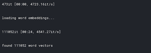
    print('loading word embeddings...')
    embeddings_index = {}
    f = open('../input/fasttext/wiki.simple.vec',encoding='utf-8')
    for line in tqdm(f):
        values = line.strip().rsplit(' ')
        word = values[0]
        coefs = np.asarray(values[1:], dtype='float32')
        embeddings_index[word] = coefs
    f.close()
    print('found %s word vectors' % len(embeddings_index))

    return embeddings_index

embeddings_index=load_fastext()

embeddings_index['london'].shape

GloVe

GloVe (global vectors for word representation) « ».

, .

word2vec, .

.
.

, .

n- .

def load_glove():
    embedding_dict = {}
    path = '../input/glove-global-vectors-for-word-representation/glove.6B.100d.txt'
    with open(path, 'r') as f:
        for line in f:
            values = line.split()
            word = values[0]
            vectors = np.asarray(values[1:], 'float32')
            embedding_dict[word] = vectors
    f.close()

    return embedding_dict

embeddings_index = load_glove()

, , GloVe.

- .

embeddings_index['london'].shape

.
.
.

, .

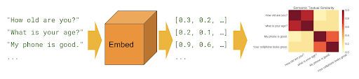
Tensorflow.

module_url = "../input/universalsentenceencoderlarge4"
# Import the Universal Sentence Encoder's TF Hub module
embed = hub.load(module_url)

sentence_list=df.question_text.values.tolist()
sentence_emb=embed(sentence_list)['outputs'].numpy()

Elmo, BERT

, .

«stick», «», «» , , .

NLP BERT , . .

, Keras .

, .

, Keras Tokenizer pad_sequences.

MAX_LEN=50
tokenizer_obj=Tokenizer()
tokenizer_obj.fit_on_texts(corpus)
sequences=tokenizer_obj.texts_to_sequences(corpus)

tweet_pad=pad_sequences(sequences,
                        maxlen=MAX_LEN,
                        truncating='post',
                        padding='post')

word_index=tokenizer_obj.word_index
print('Number of unique words:',len(word_index))

, .

def prepare_matrix(embedding_dict, emb_size=300):
    num_words = len(word_index)
    embedding_matrix = np.zeros((num_words, emb_size))

    for word, i in tqdm(word_index.items()):
        if i > num_words:
            continue

    emb_vec = embedding_dict.get(word)
    if emb_vec is not None:
        embedding_matrix[i] = emb_vec

    return embedding_matrix

trainable=False, .

def new_model(embedding_matrix):
    inp = Input(shape=(MAX_LEN,))

    x = Embedding(num_words, embedding_matrix.shape[1], weights=[embedding_matrix],
                  trainable=False)(inp)

    x = Bidirectional(
        LSTM(60, return_sequences=True, name='lstm_layer', 
             dropout=0.1, recurrent_dropout=0.1))(x)

    x = GlobalAveragePool1D()(x)
    x = Dense(1, activation="sigmoid")(x)
    model = Model(inputs=inp, outputs=x)

    model.compile(loss='binary_crossentropy',
                  optimizer='adam',
                  metrics=['accuracy'])

    return model

, , word2vec:

embeddings_index=load_word2vec()
embedding_matrix=prepare_matrix(embeddings_index)
model=new_model(embedding_matrix)

history=model.fit(X_train,y_train,
                  batch_size=8,
                  epochs=5,
                  validation_data=(X_test,y_test),
                  verbose=2)

, .

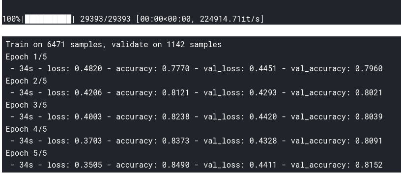
Neptune .

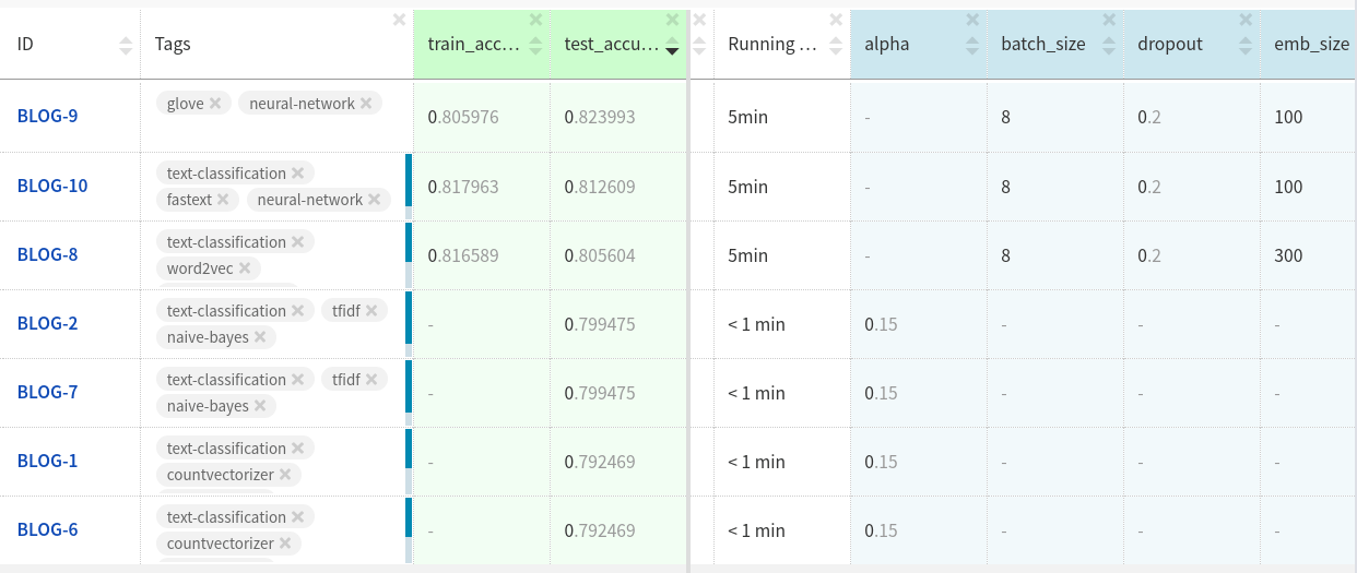
Les pièces jointes GloVe dans les jeux de données de test se sont comportées légèrement mieux que les deux autres pièces jointes.

Vous obtiendrez peut-être plus si vous personnalisez davantage le modèle et nettoyez les données.

Vous pouvez regarder les expériences ici .

Conclusion

Dans cet article, nous avons examiné et implémenté diverses méthodes de présentation des attributs de classification de texte utilisés lors de l'utilisation de petits ensembles de données.

J'espère qu'ils vous seront utiles dans vos projets.

Classification des documents: 7 approches pratiques pour les petits ensembles de données

Introduction à la classification des documents

Ensemble de données de test pour la classification

CountVectorizer

TfidfVectorizer

Word2vec

FastText

GloVe

Elmo, BERT

Conclusion

More articles: