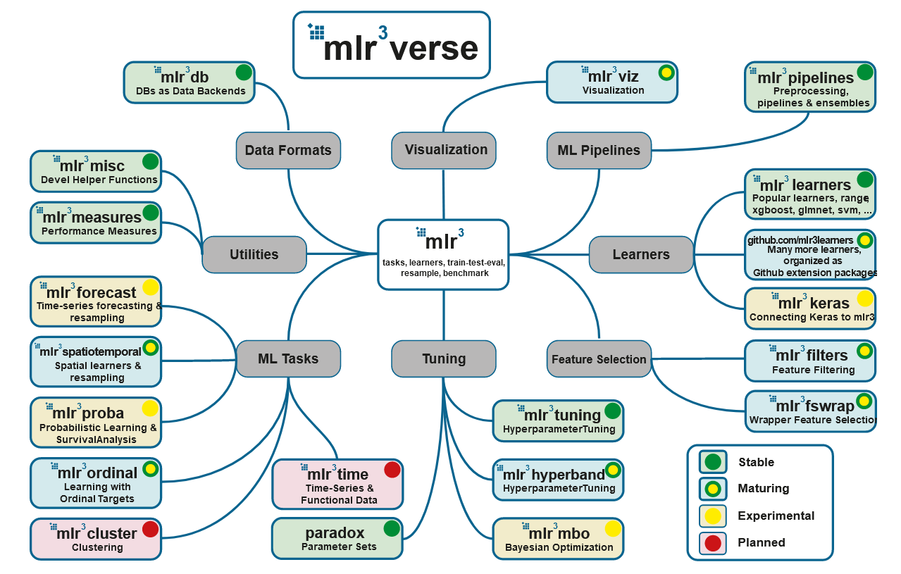
Source: https://mlr3book.mlr-org.com/
Bonjour, Habr!Dans cet article, nous considérerons l'approche la plus réfléchie de l'apprentissage automatique en langage R aujourd'hui - le package mlr3 et l'écosystème qui l'entoure. Cette approche est basée sur une POO «normale» utilisant des classes R6 et sur la représentation de toutes les opérations avec des données et des modèles sous forme de graphe de calcul. Cela vous permet de créer des pipelines rationalisés et flexibles pour les tâches d'apprentissage automatique, mais au début, cela peut sembler compliqué et déroutant. Ci-dessous, nous essaierons d'apporter de la clarté et de motiver l'utilisation de mlr3 dans vos projets.Contenu:
- Un peu d'histoire et de comparaison avec des solutions concurrentes
- Détails techniques: classes R6 et package data.table
- Les principaux composants de la ML Pipline dans mlr3
- Définition des hyperparamètres
- Présentation de l'écosystème MLR3
- Tuyaux et graphique des calculs
1.
caret — ,
caret R ( CRAN 2007 ). 2013 Applied Predictive Modeling, .
:
- ( - );
- (-), , , ;
- , caret- - ;
- — , xgboost
nrounds, max_depth, eta, gamma, colsample_bytree, min_child_weight subsample.
:
- — , . ;
- : , . recipes , ;
- - (nested resampling), caretEnsemble.
tidyverse strikes back
tidymodels, recipes ( «» , ), rsample ( ) tune ( ).
:
- «» , ;
- , embed textrecipes;
- , . ( tune);
- workflows «» .
:
- , tune . «» , ,
apply/map-; - . , 200 ;
- - .
mlr3 vs
mlr3 mlr , caret tidymodels. mlr , mlr3.
:
- R6-, data.table;
- . , ;
- API ,
learner — ; - .
:
2. : R6- data.table
mlr3 «» , R6-. R6- , . Advanced R, , .
R6- R6Class():
library(R6)

Accumulator <- R6Class("Accumulator", list(
  sum = 0,
  add = function(x = 1) {
    self$sum <- self$sum + x
    invisible(self)
  })
)
— "Accumulator".
new(), (, , ) :
x <- Accumulator$new()
, , :
x$add(4)
x$sum
#> [1] 4
R6- :
y1 <- Accumulator$new()
y2 <- y1

y1$add(10)
c(y1 = y1$sum, y2 = y2$sum)
#> y1 y2
#> 10 10
clone() ( clone(deep = TRUE) ):
y1 <- Accumulator$new()
y2 <- y1$clone()

y1$add(10)
c(y1 = y1$sum, y2 = y2$sum)
#> y1 y2
#> 10  0
, R6 mlr3.
data.table ( , data.table data.table: R). - data.table, := . , , 2 , . , , .
3. ML- mlr3

: https://mlr3book.mlr-org.com/
mlr3 :
library(mlr3)

#
task <- TaskClassif$new(id = "iris",
                        backend = iris,
                        target = "Species")
task
# <TaskClassif:iris> (150 x 5)
# * Target: Species
# * Properties: multiclass
# * Features (4):
#   - dbl (4): Petal.Length, Petal.Width, Sepal.Length, Sepal.Width

#
# learner_rpart <- mlr_learners$get("classif.rpart")
learner_rpart <- lrn("classif.rpart",
                     predict_type = "prob",
                     minsplit = 50)
learner_rpart
# <LearnerClassifRpart:classif.rpart>
# * Model: -
# * Parameters: xval=0, minsplit=50
# * Packages: rpart
# * Predict Type: prob
# * Feature types: logical, integer, numeric, factor, ordered
# * Properties: importance, missings, multiclass, selected_features, twoclass, weights

#
learner_rpart$param_set
# ParamSet:
#                id    class lower upper levels     default value
# 1:       minsplit ParamInt     1   Inf                 20    50
# 2:      minbucket ParamInt     1   Inf        <NoDefault>
# 3:             cp ParamDbl     0     1               0.01
# 4:     maxcompete ParamInt     0   Inf                  4
# 5:   maxsurrogate ParamInt     0   Inf                  5
# 6:       maxdepth ParamInt     1    30                 30
# 7:   usesurrogate ParamInt     0     2                  2
# 8: surrogatestyle ParamInt     0     1                  0
# 9:           xval ParamInt     0   Inf                 10     0

#
learner_rpart$train(task, row_ids = 1:120)
learner_rpart$model
# n= 120
#
# node), split, n, loss, yval, (yprob)
#       * denotes terminal node
#
# 1) root 120 70 setosa (0.41666667 0.41666667 0.16666667)
#   2) Petal.Length< 2.45 50  0 setosa (1.00000000 0.00000000 0.00000000) *
#   3) Petal.Length>=2.45 70 20 versicolor (0.00000000 0.71428571 0.28571429)
#     6) Petal.Length< 4.95 49  1 versicolor (0.00000000 0.97959184 0.02040816) *
#     7) Petal.Length>=4.95 21  2 virginica (0.00000000 0.09523810 0.90476190) *
: (task) (learner).
(TaskClassif , TaskRegr ..) new(). id, backend target; positive. : mlr_tasks$get("iris") tsk("iris").
mlr_learners get() train(), task , . : lrn("classif.rpart", predict_type = "prob", minsplit = 50). (predict_type = "prob") (minsplit = 50). : learner_rpart$predict_type <- "prob", learner_rpart$param_set$values$minsplit = 50.
predict_newdata():
#
preds <- learner_rpart$predict_newdata(newdata = iris[121:150, ])
preds
# <PredictionClassif> for 30 observations:
#     row_id     truth   response prob.setosa prob.versicolor prob.virginica
#          1 virginica  virginica           0       0.0952381     0.90476190
#          2 virginica versicolor           0       0.9795918     0.02040816
#          3 virginica  virginica           0       0.0952381     0.90476190
# ---
#         28 virginica  virginica           0       0.0952381     0.90476190
#         29 virginica  virginica           0       0.0952381     0.90476190
#         30 virginica  virginica           0       0.0952381     0.90476190
- 5 :
cv10 <- rsmp("cv", folds = 5)

resample_results <- resample(task, learner_rpart, cv10)
# INFO  [09:37:05.993] Applying learner 'classif.rpart' on task 'iris' (iter 1/5)
# INFO  [09:37:06.018] Applying learner 'classif.rpart' on task 'iris' (iter 2/5)
# INFO  [09:37:06.042] Applying learner 'classif.rpart' on task 'iris' (iter 3/5)
# INFO  [09:37:06.074] Applying learner 'classif.rpart' on task 'iris' (iter 4/5)
# INFO  [09:37:06.098] Applying learner 'classif.rpart' on task 'iris' (iter 5/5)

resample_results
# <ResampleResult> of 5 iterations
# * Task: iris
# * Learner: classif.rpart
# * Warnings: 0 in 0 iterations
# * Errors: 0 in 0 iterations

#    (-):
as.data.table(mlr_resamplings)
#            key        params iters
# 1:   bootstrap repeats,ratio    30
# 2:      custom                   0
# 3:          cv         folds    10
# 4:     holdout         ratio     1
# 5: repeated_cv repeats,folds   100
# 6: subsampling repeats,ratio    30
. score() resample_results, — accuracy "classif.acc" classification error "classif.ce". , get(): mlr_measures$get("classif.ce"). msrs():
resample_results$score(msrs(c("classif.acc", "classif.ce")))[, 5:10]
#
#        resampling resampling_id iteration prediction classif.acc classif.ce
# 1: <ResamplingCV>            cv         1     <list>   0.8666667 0.13333333
# 2: <ResamplingCV>            cv         2     <list>   0.9666667 0.03333333
# 3: <ResamplingCV>            cv         3     <list>   0.9333333 0.06666667
# 4: <ResamplingCV>            cv         4     <list>   0.9666667 0.03333333
# 5: <ResamplingCV>            cv         5     <list>   0.9333333 0.06666667
4.
— . , .
. paradox:
library("paradox")
searchspace <- ParamSet$new(list(
  ParamDbl$new("cp", lower = 0.001, upper = 0.1),
  ParamInt$new("minsplit", lower = 1, upper = 10)
))
searchspace
# ParamSet:
#          id    class lower upper levels     default value
# 1:       cp ParamDbl 0.001   0.1        <NoDefault>
# 2: minsplit ParamInt 1.000  10.0        <NoDefault>
ParamSet, cp minsplit; rpart .
, searchspace . tune() Tuner. . resolution, , param_resolutions, . , , .
generate_design_grid() , :
generate_design_grid(searchspace,
                     param_resolutions = c("cp" = 2, "minsplit" = 3))
# <Design> with 6 rows:
#       cp minsplit
# 1: 0.001        1
# 2: 0.001        5
# 3: 0.001       10
# 4: 0.100        1
# 5: 0.100        5
# 6: 0.100       10
: generate_design_random() generate_design_lhs() .
, . Terminator-, , ( ), . mlr3tuning:
library("mlr3tuning")

evals20 <- term("evals", n_evals = 20)
evals20
# <TerminatorEvals>
# * Parameters: n_evals=20

#
as.data.table(mlr_terminators)
#             key
# 1:   clock_time
# 2:        combo
# 3:        evals
# 4:   model_time
# 5:         none
# 6: perf_reached
# 7:   stagnation
TuningInstance:
tuning_instance <- TuningInstance$new(
  task = TaskClassif$new(id = "iris",
                        backend = iris,
                        target = "Species"),
  learner = lrn("classif.rpart",
                predict_type = "prob"),
  resampling = rsmp("cv", folds = 5),
  measures = msr("classif.ce"),
  param_set = ParamSet$new(
    list(ParamDbl$new("cp", lower = 0.001, upper = 0.1),
         ParamInt$new("minsplit", lower = 1, upper = 10)
         )
    ),
  terminator = term("evals", n_evals = 20)
)

tuning_instance
# <TuningInstance>
# * State:  Not tuned
# * Task: <TaskClassif:iris>
# * Learner: <LearnerClassifRpart:classif.rpart>
# * Measures: classif.ce
# * Resampling: <ResamplingCV>
# * Terminator: <TerminatorEvals>
# * bm_args: list()
# * n_evals: 0
# ParamSet:
#          id    class lower upper levels     default value
# 1:       cp ParamDbl 0.001   0.1        <NoDefault>
# 2: minsplit ParamInt 1.000  10.0        <NoDefault>
— Tuner, :
tuner <- tnr("grid_search",
             resolution = 5,
             batch_size = 2)

#
# as.data.table(mlr_tuners)
#              key
# 1: design_points
# 2:         gensa
# 3:   grid_search
# 4: random_search
resolution = 5, 25 . 20 , terminator = term("evals", n_evals = 20). batch_size — , . mlr3 — , .
tnr("design_points"): , ( — , mlr3 ).
, :
result <- tuner$tune(tuning_instance)
result
# NULL
, result . , tuner$tune() tuning_instance:
tuning_instance$result
# $tune_x
# $tune_x$cp
# [1] 0.001
#
# $tune_x$minsplit
# [1] 5
#
#
# $params
# $params$xval
# [1] 0
#
# $params$cp
# [1] 0.001
#
# $params$minsplit
# [1] 5
#
#
# $perf
# classif.ce
#       0.04

result <- tuning_instance$archive(unnest = "params")
result[order(classif.ce), c("cp", "minsplit", "classif.ce")]
#         cp minsplit classif.ce
#  1: 0.00100        5 0.04000000
#  2: 0.00100        3 0.04000000
#  3: 0.00100        8 0.04000000
#  4: 0.00100        1 0.04000000
#  5: 0.00100       10 0.04666667
#  6: 0.02575       10 0.06000000
#  7: 0.07525        5 0.06000000
#  8: 0.02575        8 0.06000000
#  9: 0.02575        3 0.06000000
# 10: 0.05050        1 0.06000000
# 11: 0.07525        3 0.06000000
# 12: 0.07525        1 0.06000000
# 13: 0.05050        3 0.06000000
# 14: 0.02575        5 0.06000000
# 15: 0.05050        5 0.06000000
# 16: 0.05050        8 0.06000000
# 17: 0.10000        3 0.06000000
# 18: 0.10000        8 0.06000000
# 19: 0.05050       10 0.06000000
# 20: 0.10000        1 0.06000000

library(ggplot2)
ggplot(result,
       aes(x = cp, y = classif.ce, color = as.factor(minsplit))) +
  geom_line() +
  geom_point(size = 3)

, tune():
Tuner ( batch_size);Learner Task . ResampleResult ( BenchmarkResult);Terminator , . , 1, , ;- ;
- , ( , ,
msr("classif.ce", aggregator = "median").
tuning_instance$bmr, BenchmarkResult, score() as.data.table(tuning_instance$bmr). , , ResampleResult tuning_instance$archive():
tuning_instance$archive()[1, resample_result][[1]]$score()[, 4:9]
#       learner_id     resampling resampling_id iteration prediction classif.ce
# 1: classif.rpart <ResamplingCV>            cv         1     <list> 0.06666667
# 2: classif.rpart <ResamplingCV>            cv         2     <list> 0.16666667
# 3: classif.rpart <ResamplingCV>            cv         3     <list> 0.03333333
# 4: classif.rpart <ResamplingCV>            cv         4     <list> 0.03333333
# 5: classif.rpart <ResamplingCV>            cv         5     <list> 0.00000000
, :
res <- tuning_instance$archive(unnest = "params")
res[, ce_resemples := lapply(resample_result, function(x) x$score()[, classif.ce])]
ce_resemples <- res[, .(ce_resemples = unlist(ce_resemples)), by = nr]
res[ce_resemples, on = "nr"]
5. mlr3
: mlr3, mlr3tuning paradox. , - mlr3verse:
# install.packages("mlr3verse")
library(mlr3verse)
## Loading required package: mlr3
## Loading required package: mlr3db
## Loading required package: mlr3filters
## Loading required package: mlr3learners
## Loading required package: mlr3pipelines
## Loading required package: mlr3tuning
## Loading required package: mlr3viz
## Loading required package: paradox
- mlr3db dbplyr data.table.
- mlr3filters , ( ).
- mlr3learners (
regr.glmnet, regr.kknn, regr.km, regr.lm, regr.ranger, regr.svm, regr.xgboost) (classif.glmnet, classif.kknn, classif.lda, classif.log_reg, classif.multinom, classif.naive_bayes, classif.qda, classif.ranger, classif.svm, classif.xgboost). . - mlr3pipelines (pipelines), . , , CRAN, :
remotes::install_github("https://github.com/mlr-org/mlr3pipelines"). - mlr3tuning .
- mlr3viz , .
- mlr3measures — ~40 . mlr3verse , .
, .
6.
(pipelines) , , .
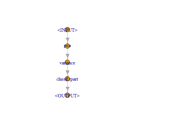
— , , — . PipeOpLearner(), — PipeOpFilter(), — PipeOp(). ( po()) :
pca <- po("pca")
filter <- po("filter",
             filter = mlr3filters::flt("variance"),
             filter.frac = 0.5)
learner_po <- po("learner",
                 learner = lrn("classif.rpart"))
%>>%:
graph <- pca %>>% filter %>>% learner_po
graph$plot()
. , :
gr <- Graph$new()$
  add_pipeop(mlr_pipeops$get("copy", outnum = 2))$
  add_pipeop(mlr_pipeops$get("scale"))$
  add_pipeop(mlr_pipeops$get("pca"))$
  add_pipeop(mlr_pipeops$get("featureunion", innum = 2))

gr$
  add_edge("copy", "scale", src_channel = 1)$
  add_edge("copy", "pca", src_channel = "output2")$
  add_edge("scale", "featureunion", dst_channel = 1)$
  add_edge("pca", "featureunion", dst_channel = 2)

gr$plot(html = FALSE)

, (po("learner", learner = lrn("classif.rpart"))). , :
glrn <- GraphLearner$new(graph)
glrn
# <GraphLearner:pca.variance.classif.rpart>
# * Model: -
# * Parameters: variance.filter.frac=0.5, variance.na.rm=TRUE, classif.rpart.xval=0
# * Packages: -
# * Predict Type: response
# * Feature types: logical, integer, numeric, character, factor, ordered, POSIXct
# * Properties: importance, missings, multiclass, oob_error, selected_features, twoclass,
#   weights
GraphLearner Learner. , Learner-, :
resample(tsk("iris"), glrn, rsmp("cv"))
# INFO  [17:17:00.358] Applying learner 'pca.variance.classif.rpart' on task 'iris' (iter 1/10)
# INFO  [17:17:00.615] Applying learner 'pca.variance.classif.rpart' on task 'iris' (iter 2/10)
# INFO  [17:17:00.881] Applying learner 'pca.variance.classif.rpart' on task 'iris' (iter 3/10)
# INFO  [17:17:01.087] Applying learner 'pca.variance.classif.rpart' on task 'iris' (iter 4/10)
# INFO  [17:17:01.303] Applying learner 'pca.variance.classif.rpart' on task 'iris' (iter 5/10)
# INFO  [17:17:01.518] Applying learner 'pca.variance.classif.rpart' on task 'iris' (iter 6/10)
# INFO  [17:17:01.716] Applying learner 'pca.variance.classif.rpart' on task 'iris' (iter 7/10)
# INFO  [17:17:01.927] Applying learner 'pca.variance.classif.rpart' on task 'iris' (iter 8/10)
# INFO  [17:17:02.129] Applying learner 'pca.variance.classif.rpart' on task 'iris' (iter 9/10)
# INFO  [17:17:02.337] Applying learner 'pca.variance.classif.rpart' on task 'iris' (iter 10/10)
# <ResampleResult> of 10 iterations
# * Task: iris
# * Learner: pca.variance.classif.rpart
# * Warnings: 0 in 0 iterations
# * Errors: 0 in 0 iterations
, issue How to deal with different preprocessing steps as hyperparameters:
gr <- pipeline_branch(list(pca = po("pca"), nothing = po("nop")))
gr$plot()

caret tidymodels !
, mlr3. mlr3 book .