Cualquier actividad genera datos. Hagas lo que hagas, probablemente tengas en tus manos un almacén de información útil en bruto, o al menos acceso a su fuente.
Hoy el ganador es el que toma decisiones basadas en datos objetivos. Las habilidades del analista son más relevantes que nunca, y la disponibilidad de las herramientas necesarias a la mano le permite estar siempre un paso adelante. Esta es una ayuda en la aparición de este artículo.
¿Tienes tu propio negocio? O tal vez ... aunque, no importa. El proceso de minería de datos es interminable y emocionante. E incluso solo cavando bien en Internet, puede encontrar un campo para la actividad.
Esto es lo que tenemos hoy: una base de datos de distribución XML no oficial para RuTracker.ORG. La base de datos se actualiza cada seis meses y contiene información sobre todas las distribuciones para el historial de la existencia de este rastreador de torrents.
¿Qué puede decirle a los dueños del rutracker? ¿Y los cómplices directos de la piratería en Internet? ¿O un usuario común aficionado al anime, por ejemplo?
¿Entiendes lo que quiero decir?
Descargo de responsabilidad Pila - R, Clickhouse, Dataiku
Cualquier análisis pasa por varias etapas principales: extracción de datos, su preparación y estudio de datos (visualización). Cada etapa tiene su propia herramienta. Porque la pila de hoy:
- R. , Python. dplyr ggplot2. – .
- Clickhouse. . : “clickhouse ” “ ”. , . .
- Dataiku. , -.
: Dataiku . 3 . .
, , , . dataiku .
Big Data – big problems
xml– 5 . – rutracker.org, (2005 .) 2019 . 15 !
R Studio – ! . , .
, R. Big Data, Clickhouse … , xml–. . .
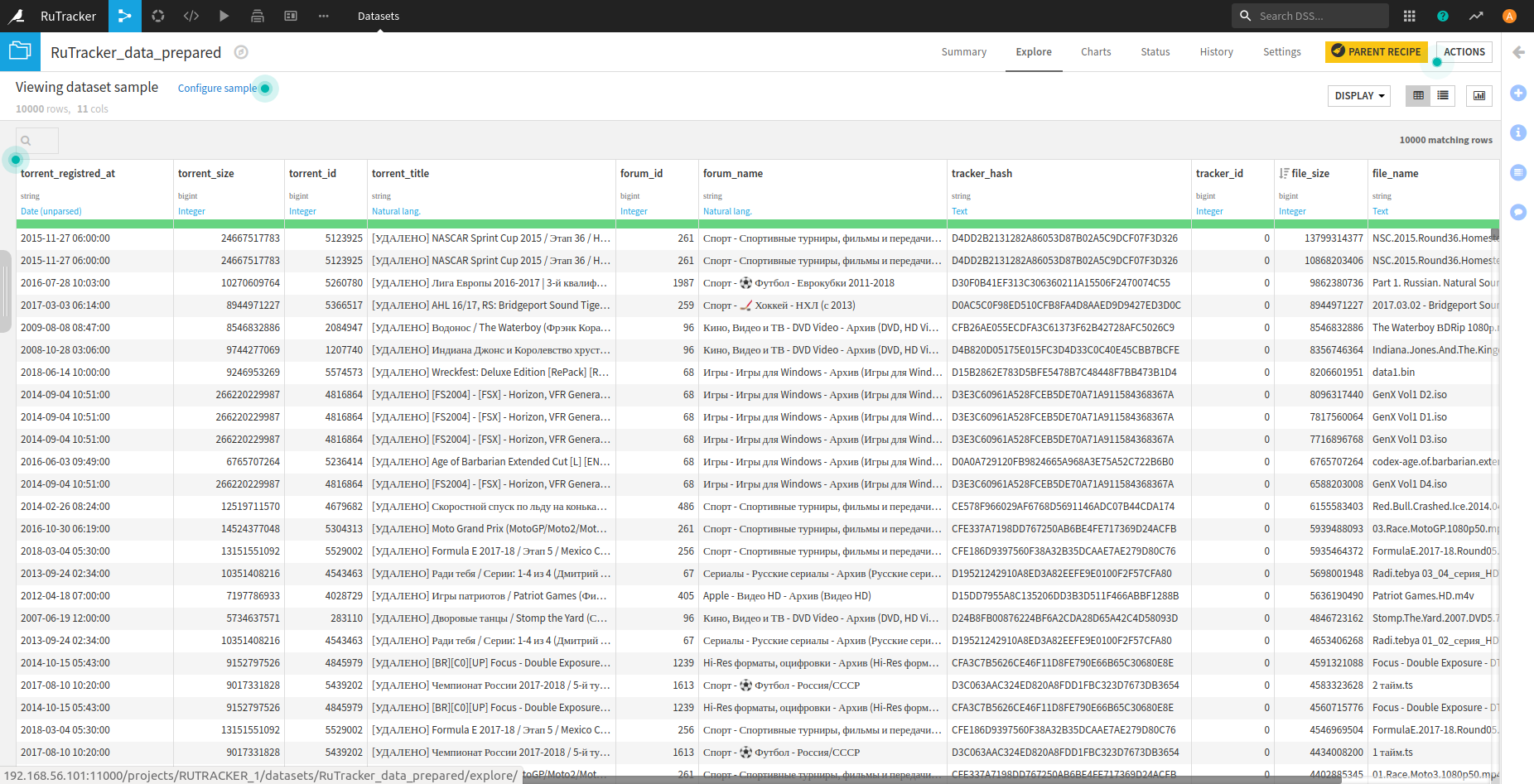
. Dataiku DSS . – 10 000 . . , . , 200 000 .
, . .

. : content — json.
content, . – .
recipe — . , . json .
. , , + dataiku.
recipe, — .
csv Clickhouse.
Clickhouse 15 rutracker-a.
?
SELECT ROUND(uniq(torrent_id) / 1000000, 2) AS Count_M
FROM rutracker

┌─Count_M─┐
│    1.46 │
└─────────┘
1 rows in set. Elapsed: 0.247 sec. Processed 25.51 million rows, 204.06 MB (103.47 million rows/s., 827.77 MB/s.)
1.5 25 . 0.3 ! .
, , .
SELECT COUNT(*) AS Count
FROM rutracker
WHERE (file_ext = 'epub') OR (file_ext = 'fb2') OR (file_ext = 'mobi')

┌──Count─┐
│ 333654 │
└────────┘
1 rows in set. Elapsed: 0.435 sec. Processed 25.51 million rows, 308.79 MB (58.64 million rows/s., 709.86 MB/s.)
300 — ! , . .
SELECT ROUND(SUM(file_size) / 1000000000, 2) AS Total_size_GB
FROM rutracker
WHERE (file_ext = 'epub') OR (file_ext = 'fb2') OR (file_ext = 'mobi')

┌─Total_size_GB─┐
│        625.75 │
└───────────────┘
1 rows in set. Elapsed: 0.296 sec. Processed 25.51 million rows, 344.32 MB (86.24 million rows/s., 1.16 GB/s.)
– 25 . , ?
R
R. , DBI ( ). Clickhouse.
Rlibrary(DBI) # , ... Clickhouse
library(dplyr) # %>%
#
library(ggplot2)
library(ggrepel)
library(cowplot)
library(scales)
library(ggrepel)
# localhost:9000
connection <- dbConnect(RClickhouse::clickhouse(), host="localhost", port = 9000)
, . dplyr .
? rutracker.org .
Ryears_stat <- dbGetQuery(connection,
"SELECT
round(COUNT(*)/1000000, 2) AS Files,
round(uniq(torrent_id)/1000, 2) AS Torrents,
toYear(torrent_registred_at) AS Year
FROM rutracker
GROUP BY Year")
ggplot(years_stat, aes(as.factor(Year), as.double(Files))) +
geom_bar(stat = 'identity', fill = "darkblue", alpha = 0.8)+
theme_minimal() +
labs(title = " RuTracker", subtitle = " 2005 - 2019\n")+
theme(axis.text.x = element_text(angle=90, vjust = 0.5),
axis.text.y = element_text(),
axis.title.y = element_blank(),
axis.title.x = element_blank(),
panel.grid.major.x = element_blank(),
panel.grid.major.y = element_line(size = 0.9),
panel.grid.minor.y = element_line(size = 0.4),
plot.title = element_text(vjust = 3, hjust = 0, family = "sans", size = 16, color = "#101010", face = "bold"),
plot.caption = element_text(vjust = 3, hjust = 0, family = "sans", size = 12, color = "#101010", face = "bold"),
plot.margin = unit(c(1,0.5,1,0.5), "cm"))+
scale_y_continuous(labels = number_format(accuracy = 1, suffix = " "))
ggplot(years_stat, aes(as.factor(Year), as.integer(Torrents))) +
geom_bar(stat = 'identity', fill = "#008b8b", alpha = 0.8)+
theme_minimal() +
labs(title = " RuTracker", subtitle = " 2005 - 2019\n", caption = "* ")+
theme(axis.text.x = element_text(angle=90, vjust = 0.5),
axis.text.y = element_text(),
axis.title.y = element_blank(),
axis.title.x = element_blank(),
panel.grid.major.x = element_blank(),
panel.grid.major.y = element_line(size = 0.9),
panel.grid.minor.y = element_line(size = 0.4),
plot.title = element_text(vjust = 3, hjust = 0, family = "sans", size = 16, color = "#101010", face = "bold"),
plot.caption = element_text(vjust = -3, hjust = 1, family = "sans", size = 9, color = "grey60", face = "plain"),
plot.margin = unit(c(1,0.5,1,0.5), "cm")) +
scale_y_continuous(labels = number_format(accuracy = 1, suffix = " "))
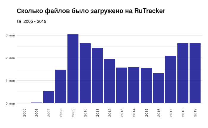
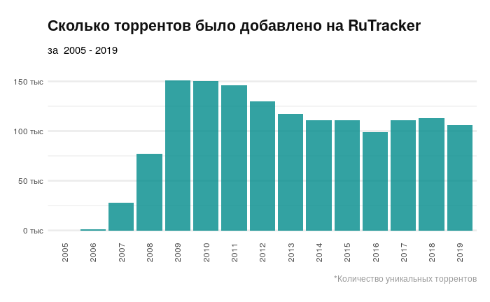
2016 . , 2016 rutracker.org . , .
, . , .
.
Rextention_stat <- dbGetQuery(connection,
"SELECT toYear(torrent_registred_at) AS Year,
COUNT(tracker_id)/1000 AS Count,
ROUND(SUM(file_size)/1000000000000, 2) AS Total_Size_TB,
file_ext
FROM rutracker
GROUP BY Year, file_ext
ORDER BY Year, Count")
#
TopExt <- function(x, n) {
res_tab <- NULL
# 2005 2006, ..
for (i in (3:15)) {
res_tab <-bind_rows(list(res_tab,
extention_stat %>% filter(Year == x[i]) %>%
arrange(desc(Count), desc(Total_Size_TB)) %>%
head(n)
))
}
return(res_tab)
}
years_list <- unique(extention_stat$Year)
ext_data <- TopExt(years_list, 5)
ggplot(ext_data, aes(as.factor(Year), as.integer(Count), fill = file_ext)) +
geom_bar(stat = "identity",position="dodge2", alpha =0.8, width = 1)+
theme_minimal() +
labs(title = " RuTracker",
subtitle = " 2005 - 2019\n",
caption = "* -5 ", fill = "") +
theme(axis.text.x = element_text(angle=90, vjust = 0.5),
axis.text.y = element_text(),
axis.title.y = element_blank(),
axis.title.x = element_blank(),
panel.grid.major.x = element_blank(),
panel.grid.major.y = element_line(size = 0.9),
panel.grid.minor.y = element_line(size = 0.4),
legend.title = element_text(vjust = 1, hjust = -1, family = "sans", size = 9, color = "#101010", face = "plain"),
legend.position = "top",
plot.title = element_text(vjust = 3, hjust = 0, family = "sans", size = 16, color = "#101010", face = "bold"),
plot.caption = element_text(vjust = -4, hjust = 1, family = "sans", size = 9, color = "grey60", face = "plain"),
plot.margin = unit(c(1,0.5,1,0.5), "cm")) +
scale_y_continuous(labels = number_format(accuracy = 0.5, scale = (1/1000), suffix = " "))+guides(fill=guide_legend(nrow=1))
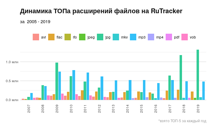
. . .
rutracker-a. .
Rchapter_stat <- dbGetQuery(connection,
"SELECT
substring(forum_name, 1, position(forum_name, ' -')) Chapter,
uniq(torrent_id) AS Count,
ROUND(median(file_size)/1000000, 2) AS Median_Size_MB,
ROUND(max(file_size)/1000000000) AS Max_Size_GB,
ROUND(SUM(file_size)/1000000000000) AS Total_Size_TB
FROM rutracker WHERE Chapter NOT LIKE('\"%')
GROUP BY Chapter
ORDER BY Count DESC")
chapter_stat$Count <- as.integer(chapter_stat$Count)
#
AggChapter2 <- function(Chapter){
var_ch <- str(Chapter)
res = NULL
for(i in (1:22)){
select_str <-paste0(
"SELECT
toYear(torrent_registred_at) AS Year,
substring(forum_name, 1, position(forum_name, ' -')) Chapter,
uniq(torrent_id)/1000 AS Count,
ROUND(median(file_size)/1000000, 2) AS Median_Size_MB,
ROUND(max(file_size)/1000000000,2) AS Max_Size_GB,
ROUND(SUM(file_size)/1000000000000,2) AS Total_Size_TB
FROM rutracker
WHERE Chapter LIKE('", Chapter[i], "%')
GROUP BY Year, Chapter
ORDER BY Year")
res <-bind_rows(list(res, dbGetQuery(connection, select_str)))
}
return(res)
}
chapters_data <- AggChapter2(chapter_stat$Chapter)
chapters_data$Chapter <- as.factor(chapters_data$Chapter)
chapters_data$Count <- as.numeric(chapters_data$Count)
chapters_data %>% group_by(Chapter)%>%
ggplot(mapping = aes(x = reorder(Chapter, Total_Size_TB), y = Total_Size_TB))+
geom_bar(stat = "identity", fill="darkblue", alpha =0.8)+
theme(panel.grid.major.x = element_line(colour="grey60", linetype="dashed"))+
xlab('\n') + theme_minimal() +
labs(title = "C RuTracker-",
subtitle = " 2019\n")+
theme(axis.text.x = element_text(),
axis.text.y = element_text(family = "sans", size = 9, color = "#101010", hjust = 1, vjust = 0.5),
axis.title.y = element_text(vjust = 2.5, hjust = 0, family = "sans", size = 9, color = "grey40", face = "plain"),
axis.title.x = element_blank(),
axis.line.x = element_line(color = "grey60", size = 0.1, linetype = "solid"),
panel.grid.major.y = element_blank(),
panel.grid.major.x = element_line(size = 0.7, linetype = "solid"),
panel.grid.minor.x = element_line(size = 0.4, linetype = "solid"),
plot.title = element_text(vjust = 3, hjust = 1, family = "sans", size = 16, color = "#101010", face = "bold"),
plot.subtitle = element_text(vjust = 2, hjust = 1, family = "sans", size = 12, color = "#101010", face = "plain"),
plot.caption = element_text(vjust = -3, hjust = 1, family = "sans", size = 9, color = "grey60", face = "plain"),
plot.margin = unit(c(1,0.5,1,0.5), "cm"))+
scale_y_continuous(labels = number_format(accuracy = 1, suffix = " "))+
coord_flip()
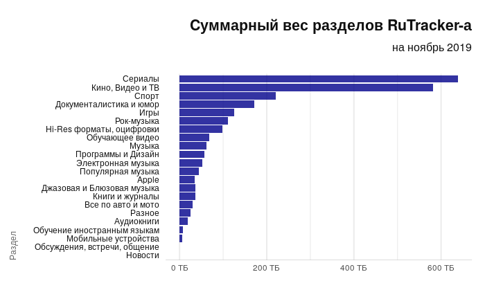
. — — . , . , Apple.
Rchapters_data %>% group_by(Chapter)%>%
ggplot(mapping = aes(x = reorder(Chapter, Count), y = Count))+
geom_bar(stat = "identity", fill="#008b8b", alpha =0.8)+
theme(panel.grid.major.x = element_line(colour="grey60", linetype="dashed"))+
xlab('') + theme_minimal() +
labs(title = " RuTracker-",
subtitle = " 2019\n")+
theme(axis.text.x = element_text(),
axis.text.y = element_text(family = "sans", size = 9, color = "#101010", hjust = 1, vjust = 0.5),
axis.title.y = element_text(vjust = 3.5, hjust = 0, family = "sans", size = 9, color = "grey40", face = "plain"),
axis.title.x = element_blank(),
axis.line.x = element_line(color = "grey60", size = 0.1, linetype = "solid"),
panel.grid.major.y = element_blank(),
panel.grid.major.x = element_line(size = 0.7, linetype = "solid"),
panel.grid.minor.x = element_line(size = 0.4, linetype = "solid"),
plot.title = element_text(vjust = 3, hjust = 1, family = "sans", size = 16, color = "#101010", face = "bold"),
plot.subtitle = element_text(vjust = 2, hjust = 1, family = "sans", size = 12, color = "#101010", face = "plain"),
plot.caption = element_text(vjust = -3, hjust = 1, family = "sans", size = 9, color = "grey60", face = "plain"),
plot.margin = unit(c(1,0.5,1,0.5), "cm"))+
scale_y_continuous(limits = c(0, 300), labels = number_format(accuracy = 1, suffix = " "))+
coord_flip()
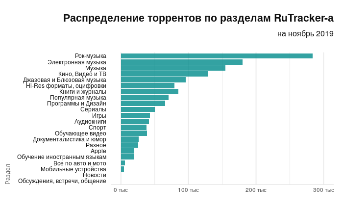
, , : -.
~15 .
Rlibrary("RColorBrewer")
getPalette = colorRampPalette(brewer.pal(19, "Spectral"))
chapters_data %>% #filter(Chapter %in% chapter_stat$Chapter[c(4,6,7,9:20)])%>%
filter(!Chapter %in% chapter_stat$Chapter[c(16, 21, 22)])%>%
filter(Year>=2007)%>%
ggplot(mapping = aes(x = Year, y = Count, fill = as.factor(Chapter)))+
geom_area(alpha =0.8, position = "fill")+
theme_minimal() +
labs(title = " -",
subtitle = " ~15 ", fill = "")+
theme(axis.text.x = element_text(vjust = 0.5),
axis.text.y = element_blank(),
axis.title.y = element_blank(),
axis.title.x = element_blank(),
panel.grid.major.x = element_blank(),
panel.grid.major.y = element_line(size = 0.9),
panel.grid.minor.y = element_line(size = 0.4),
plot.title = element_text(vjust = 3, hjust = 0, family = "sans", size = 16, color = "#101010", face = "bold"),
plot.caption = element_text(vjust = -3, hjust = 1, family = "sans", size = 9, color = "grey60", face = "plain"),
plot.margin = unit(c(1,1,1,1), "cm")) +
scale_x_continuous(breaks = c(2008, 2010, 2012, 2014, 2016, 2018),expand=c(0,0)) +
scale_fill_manual(values = getPalette(19))
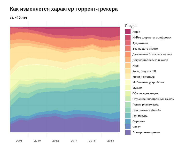
- — . — Apple , .
. .
, Rutracker-a. - rutracker.org.
Runique_torr_per_day <- dbGetQuery(connection,
"SELECT toDate(torrent_registred_at) AS date,
uniq(torrent_id) AS count
FROM rutracker
GROUP BY date
ORDER BY date")
unique_torr_per_day %>%
ggplot(aes(format(date, "%Y"), format(date, "%j"), fill = as.numeric(count)))+
geom_tile() +
theme_minimal() +
labs(title = " RuTracker-a",
subtitle = " ~15 \n\n",
fill = "- \n")+
theme(axis.text.x = element_text(vjust = 0.5),
axis.text.y = element_text(),
axis.title.y = element_blank(),
axis.title.x = element_blank(),
panel.grid.major.y = element_blank(),
panel.grid.major.x = element_line(size = 0.9),
panel.grid.minor.x = element_line(size = 0.4),
legend.title = element_text(vjust = 0.7, hjust = -1, family = "sans", size = 10, color = "#101010", face = "plain"),
legend.position = c(0.88, 1.30),
legend.direction = "horizontal",
plot.title = element_text(vjust = 3, hjust = 0, family = "sans", size = 16, color = "#101010", face = "bold"),
plot.caption = element_text(vjust = -3, hjust = 1, family = "sans", size = 9, color = "grey60", face = "plain"),
plot.margin = unit(c(1,1,1,1), "cm"))+ coord_flip(clip = "off") +
scale_y_discrete(breaks = c(format(as.Date("2007-01-15"), "%j"),
format(as.Date("2007-02-15"), "%j"),
format(as.Date("2007-03-15"), "%j"),
format(as.Date("2007-04-15"), "%j"),
format(as.Date("2007-05-15"), "%j"),
format(as.Date("2007-06-15"), "%j"),
format(as.Date("2007-07-15"), "%j"),
format(as.Date("2007-08-15"), "%j"),
format(as.Date("2007-09-15"), "%j"),
format(as.Date("2007-10-15"), "%j"),
format(as.Date("2007-11-15"), "%j"),
format(as.Date("2007-12-15"), "%j")),
labels = c("", "", "", "", "", "","", "", "", "","",""), position = 'right') +
scale_fill_gradientn(colours = c("#155220", "#c6e48b")) +
annotate(geom = "curve", x = 16.5, y = 119, xend = 13, yend = 135,
curvature = .3, color = "grey15", arrow = arrow(length = unit(2, "mm"))) +
annotate(geom = "text", x = 16, y = 45,
label = " « » \n",
hjust = "left", vjust = -0.75, color = "grey25") +
guides(x.sec = guide_axis_label_trans(~.x)) +
annotate("rect", xmin = 11.5, xmax = 12.5, ymin = 1, ymax = 366,
alpha = .0, colour = "white", size = 0.1) +
geom_segment(aes(x = 11.5, y = 25, xend = 12.5, yend = 25, colour = "segment"),
show.legend = FALSE)
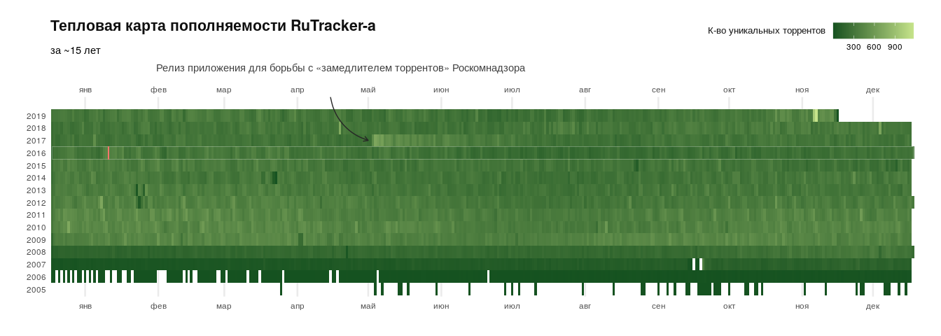
2017 . (. GitHub ). 2016 , . .
. . – .
, content , , , 15 .
Dataiku
, : , , , .
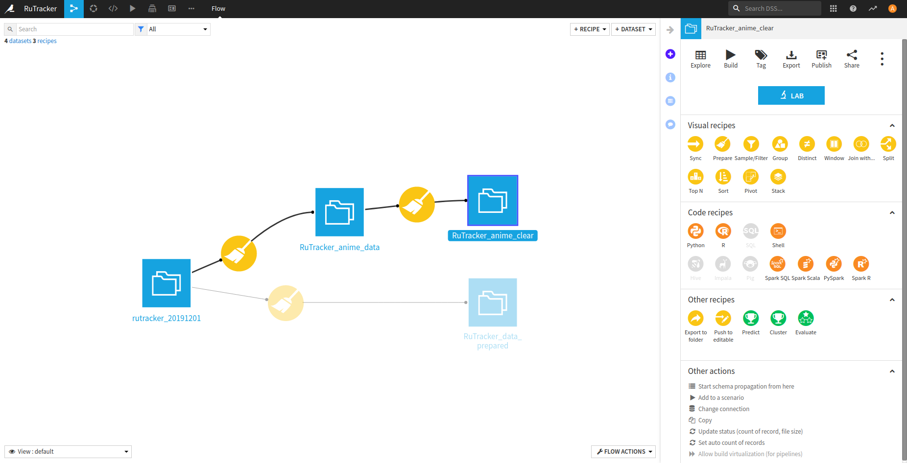
, -. . – .
– .
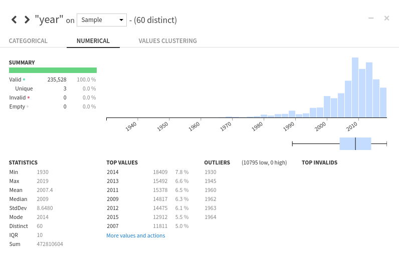
: rutracker.org , , — 60. 2009 — 2014 .
. , , . .
, . .

, dataiku — . , , (R, Python), . .
, RuTracker, : , . . , . .
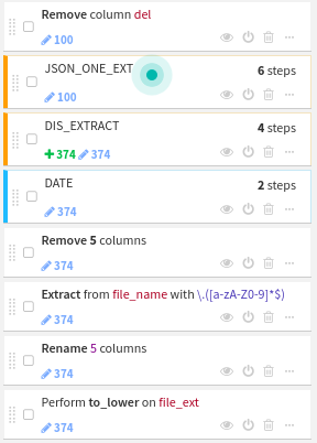
UPD: , recipe dataiku.
Condicionalmente, la receta dada en este artículo se puede dividir en dos partes: preparación de datos para análisis en R y preparación de datos sobre anime para análisis directamente en la plataforma.
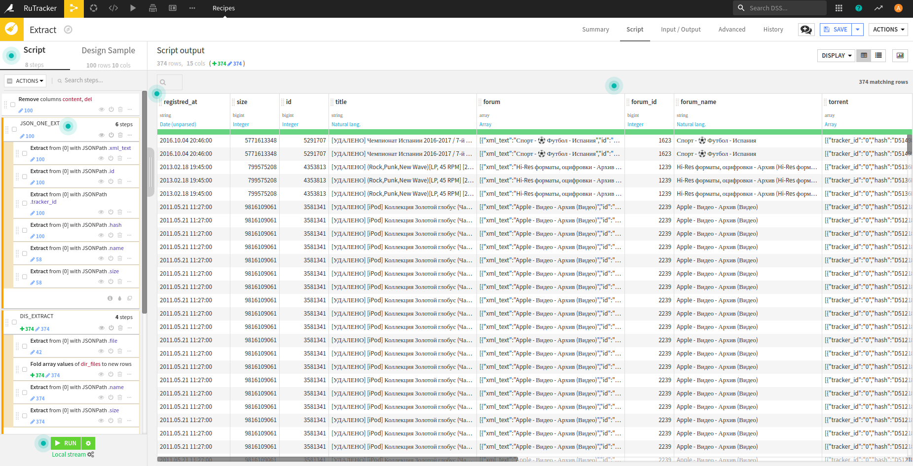
Etapa de preparación para el análisis en Rjson- .
json-. .
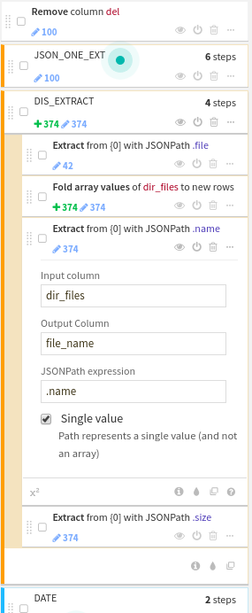
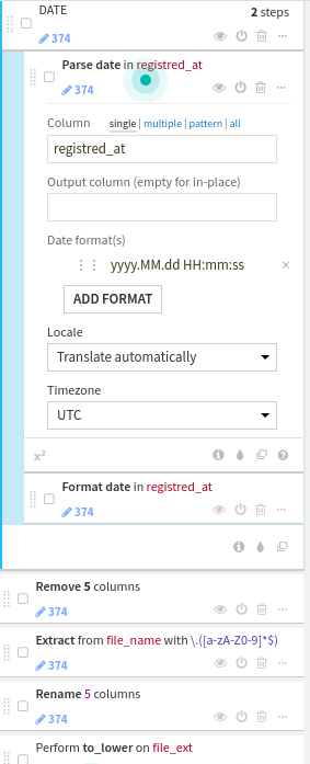
timestamp .
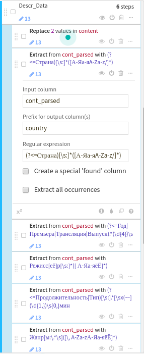
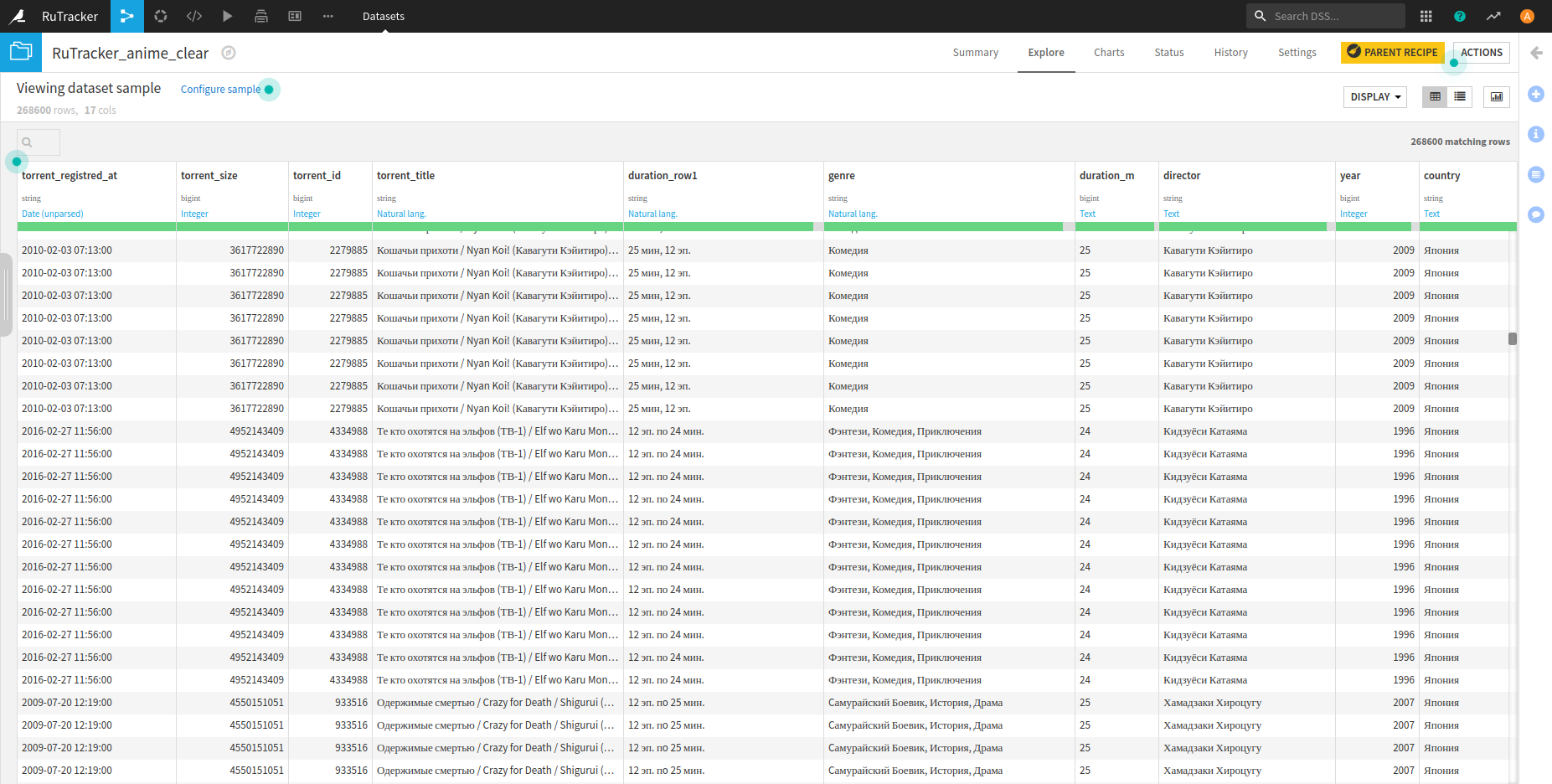
Etapa de preparación de datos de anime, , . content — Descr_Data.
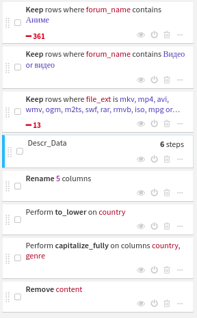
contentregexp , , , . , regexp dataiku .