💉 👩🏿‍🔧 👆🏼 Aprendizaje automático en lenguaje R usando el paquete mlr3 🉐 🧚🏿 🚴🏿

Hola Habr!

En esta publicación, consideraremos el enfoque más reflexivo para el aprendizaje automático en el lenguaje R hoy: el paquete mlr3 y el ecosistema que lo rodea. Este enfoque se basa en la OOP "normal" utilizando clases R6 y en representar todas las operaciones con datos y modelos en forma de un gráfico de cálculo. Esto le permite crear tuberías optimizadas y flexibles para las tareas de aprendizaje automático, pero al principio puede parecer complicado y confuso. A continuación intentaremos aportar algo de claridad y motivarnos para usar mlr3 en sus proyectos.

Contenido:

1.

caret — ,

caret R ( CRAN 2007 ). 2013 Applied Predictive Modeling, .

( - );
(-), , , ;
, caret- - ;
— , xgboost nrounds, max_depth, eta, gamma, colsample_bytree, min_child_weight subsample.

— , . ;
: , . recipes , ;
- (nested resampling), caretEnsemble.

tidyverse strikes back

tidymodels, recipes ( «» , ), rsample ( ) tune ( ).

«» , ;
, embed textrecipes;
, . ( tune);
workflows «» .

, tune . «» , , apply/map-;
. , 200 ;
- .

mlr3 vs

mlr3 mlr , caret tidymodels. mlr , mlr3.

R6-, data.table;
. , ;
API , learner — ;
.

: , ( ), ;
.

2. : R6- data.table

mlr3 «» , R6-. R6- , . Advanced R, , .

R6- R6Class():

library(R6)

Accumulator <- R6Class("Accumulator", list(
  sum = 0,
  add = function(x = 1) {
    self$sum <- self$sum + x 
    invisible(self)
  })
)

— "Accumulator".

new(), (, , ) :

x <- Accumulator$new()

, , :

x$add(4) 
x$sum
#> [1] 4

R6- :

y1 <- Accumulator$new() 
y2 <- y1

y1$add(10)
c(y1 = y1$sum, y2 = y2$sum)
#> y1 y2 
#> 10 10

clone() ( clone(deep = TRUE) ):

y1 <- Accumulator$new() 
y2 <- y1$clone()

y1$add(10)
c(y1 = y1$sum, y2 = y2$sum)
#> y1 y2 
#> 10  0

, R6 mlr3.

data.table ( , data.table data.table: R). - data.table, := . , , 2 , . , , .

3. ML- mlr3

: https://mlr3book.mlr-org.com/

mlr3 :

library(mlr3)

# 
task <- TaskClassif$new(id = "iris", 
                        backend = iris, 
                        target = "Species")
task
# <TaskClassif:iris> (150 x 5)
# * Target: Species
# * Properties: multiclass
# * Features (4):
#   - dbl (4): Petal.Length, Petal.Width, Sepal.Length, Sepal.Width

# 
# learner_rpart <- mlr_learners$get("classif.rpart")
learner_rpart <- lrn("classif.rpart", 
                     predict_type = "prob", 
                     minsplit = 50)
learner_rpart
# <LearnerClassifRpart:classif.rpart>
# * Model: -
# * Parameters: xval=0, minsplit=50
# * Packages: rpart
# * Predict Type: prob
# * Feature types: logical, integer, numeric, factor, ordered
# * Properties: importance, missings, multiclass, selected_features, twoclass, weights

#  
learner_rpart$param_set
# ParamSet: 
#                id    class lower upper levels     default value
# 1:       minsplit ParamInt     1   Inf                 20    50
# 2:      minbucket ParamInt     1   Inf        <NoDefault>      
# 3:             cp ParamDbl     0     1               0.01      
# 4:     maxcompete ParamInt     0   Inf                  4      
# 5:   maxsurrogate ParamInt     0   Inf                  5      
# 6:       maxdepth ParamInt     1    30                 30      
# 7:   usesurrogate ParamInt     0     2                  2      
# 8: surrogatestyle ParamInt     0     1                  0      
# 9:           xval ParamInt     0   Inf                 10     0

# 
learner_rpart$train(task, row_ids = 1:120) 
learner_rpart$model
# n= 120 
# 
# node), split, n, loss, yval, (yprob)
#       * denotes terminal node
# 
# 1) root 120 70 setosa (0.41666667 0.41666667 0.16666667)  
#   2) Petal.Length< 2.45 50  0 setosa (1.00000000 0.00000000 0.00000000) *
#   3) Petal.Length>=2.45 70 20 versicolor (0.00000000 0.71428571 0.28571429)  
#     6) Petal.Length< 4.95 49  1 versicolor (0.00000000 0.97959184 0.02040816) *
#     7) Petal.Length>=4.95 21  2 virginica (0.00000000 0.09523810 0.90476190) *

: (task) (learner).

(TaskClassif , TaskRegr ..) new(). id, backend target; positive. : mlr_tasks$get("iris") tsk("iris").

mlr_learners get() train(), task , . : lrn("classif.rpart", predict_type = "prob", minsplit = 50). (predict_type = "prob") (minsplit = 50). : learner_rpart$predict_type <- "prob", learner_rpart$param_set$values$minsplit = 50.

predict_newdata():

#    
preds <- learner_rpart$predict_newdata(newdata = iris[121:150, ])
preds
# <PredictionClassif> for 30 observations:
#     row_id     truth   response prob.setosa prob.versicolor prob.virginica
#          1 virginica  virginica           0       0.0952381     0.90476190
#          2 virginica versicolor           0       0.9795918     0.02040816
#          3 virginica  virginica           0       0.0952381     0.90476190
# ---                                                                       
#         28 virginica  virginica           0       0.0952381     0.90476190
#         29 virginica  virginica           0       0.0952381     0.90476190
#         30 virginica  virginica           0       0.0952381     0.90476190

- 5 :

cv10 <- rsmp("cv", folds = 5)

resample_results <- resample(task, learner_rpart, cv10)
# INFO  [09:37:05.993] Applying learner 'classif.rpart' on task 'iris' (iter 1/5) 
# INFO  [09:37:06.018] Applying learner 'classif.rpart' on task 'iris' (iter 2/5) 
# INFO  [09:37:06.042] Applying learner 'classif.rpart' on task 'iris' (iter 3/5) 
# INFO  [09:37:06.074] Applying learner 'classif.rpart' on task 'iris' (iter 4/5) 
# INFO  [09:37:06.098] Applying learner 'classif.rpart' on task 'iris' (iter 5/5) 

resample_results
# <ResampleResult> of 5 iterations
# * Task: iris
# * Learner: classif.rpart
# * Warnings: 0 in 0 iterations
# * Errors: 0 in 0 iterations

#    (-):
as.data.table(mlr_resamplings)
#            key        params iters
# 1:   bootstrap repeats,ratio    30
# 2:      custom                   0
# 3:          cv         folds    10
# 4:     holdout         ratio     1
# 5: repeated_cv repeats,folds   100
# 6: subsampling repeats,ratio    30

. score() resample_results, — accuracy "classif.acc" classification error "classif.ce". , get(): mlr_measures$get("classif.ce"). msrs():

resample_results$score(msrs(c("classif.acc", "classif.ce")))[, 5:10]
#   
#        resampling resampling_id iteration prediction classif.acc classif.ce
# 1: <ResamplingCV>            cv         1     <list>   0.8666667 0.13333333
# 2: <ResamplingCV>            cv         2     <list>   0.9666667 0.03333333
# 3: <ResamplingCV>            cv         3     <list>   0.9333333 0.06666667
# 4: <ResamplingCV>            cv         4     <list>   0.9666667 0.03333333
# 5: <ResamplingCV>            cv         5     <list>   0.9333333 0.06666667

4.

— . , .

. paradox:

library("paradox")
searchspace <- ParamSet$new(list(
  ParamDbl$new("cp", lower = 0.001, upper = 0.1),
  ParamInt$new("minsplit", lower = 1, upper = 10)
))
searchspace
# ParamSet: 
#          id    class lower upper levels     default value
# 1:       cp ParamDbl 0.001   0.1        <NoDefault>      
# 2: minsplit ParamInt 1.000  10.0        <NoDefault>

ParamSet, cp minsplit; rpart .

, searchspace . tune() Tuner. . resolution, , param_resolutions, . , , .

generate_design_grid() , :

generate_design_grid(searchspace, 
                     param_resolutions = c("cp" = 2, "minsplit" = 3))
# <Design> with 6 rows:
#       cp minsplit
# 1: 0.001        1
# 2: 0.001        5
# 3: 0.001       10
# 4: 0.100        1
# 5: 0.100        5
# 6: 0.100       10

: generate_design_random() generate_design_lhs() .

, . Terminator-, , ( ), . mlr3tuning:

library("mlr3tuning")

evals20 <- term("evals", n_evals = 20)
evals20
# <TerminatorEvals>
# * Parameters: n_evals=20

#  
as.data.table(mlr_terminators)
#             key
# 1:   clock_time
# 2:        combo
# 3:        evals
# 4:   model_time
# 5:         none
# 6: perf_reached
# 7:   stagnation

TuningInstance:

tuning_instance <- TuningInstance$new(
  task = TaskClassif$new(id = "iris", 
                        backend = iris, 
                        target = "Species"),
  learner = lrn("classif.rpart", 
                predict_type = "prob"),
  resampling = rsmp("cv", folds = 5),
  measures = msr("classif.ce"),
  param_set = ParamSet$new(
    list(ParamDbl$new("cp", lower = 0.001, upper = 0.1),
         ParamInt$new("minsplit", lower = 1, upper = 10)
         )
    ),
  terminator = term("evals", n_evals = 20)
)

tuning_instance
# <TuningInstance>
# * State:  Not tuned
# * Task: <TaskClassif:iris>
# * Learner: <LearnerClassifRpart:classif.rpart>
# * Measures: classif.ce
# * Resampling: <ResamplingCV>
# * Terminator: <TerminatorEvals>
# * bm_args: list()
# * n_evals: 0
# ParamSet: 
#          id    class lower upper levels     default value
# 1:       cp ParamDbl 0.001   0.1        <NoDefault>      
# 2: minsplit ParamInt 1.000  10.0        <NoDefault>

— Tuner, :

tuner <- tnr("grid_search", 
             resolution = 5, 
             batch_size = 2)

#  
# as.data.table(mlr_tuners)
#              key
# 1: design_points
# 2:         gensa
# 3:   grid_search
# 4: random_search

resolution = 5, 25 . 20 , terminator = term("evals", n_evals = 20). batch_size — , . mlr3 — , .

tnr("design_points"): , ( — , mlr3 ).

, :

result <- tuner$tune(tuning_instance)
result
# NULL

, result . , tuner$tune() tuning_instance:

tuning_instance$result
# $tune_x
# $tune_x$cp
# [1] 0.001
# 
# $tune_x$minsplit
# [1] 5
# 
# 
# $params
# $params$xval
# [1] 0
# 
# $params$cp
# [1] 0.001
# 
# $params$minsplit
# [1] 5
# 
# 
# $perf
# classif.ce 
#       0.04 

result <- tuning_instance$archive(unnest = "params")
result[order(classif.ce), c("cp", "minsplit", "classif.ce")]
#         cp minsplit classif.ce
#  1: 0.00100        5 0.04000000
#  2: 0.00100        3 0.04000000
#  3: 0.00100        8 0.04000000
#  4: 0.00100        1 0.04000000
#  5: 0.00100       10 0.04666667
#  6: 0.02575       10 0.06000000
#  7: 0.07525        5 0.06000000
#  8: 0.02575        8 0.06000000
#  9: 0.02575        3 0.06000000
# 10: 0.05050        1 0.06000000
# 11: 0.07525        3 0.06000000
# 12: 0.07525        1 0.06000000
# 13: 0.05050        3 0.06000000
# 14: 0.02575        5 0.06000000
# 15: 0.05050        5 0.06000000
# 16: 0.05050        8 0.06000000
# 17: 0.10000        3 0.06000000
# 18: 0.10000        8 0.06000000
# 19: 0.05050       10 0.06000000
# 20: 0.10000        1 0.06000000

library(ggplot2)
ggplot(result, 
       aes(x = cp, y = classif.ce, color = as.factor(minsplit))) +
  geom_line() + 
  geom_point(size = 3)

, tune():

Tuner ( batch_size);
Learner Task . ResampleResult ( BenchmarkResult);
Terminator , . , 1, , ;
;
, ( , , msr("classif.ce", aggregator = "median").

tuning_instance$bmr, BenchmarkResult, score() as.data.table(tuning_instance$bmr). , , ResampleResult tuning_instance$archive():

tuning_instance$archive()[1, resample_result][[1]]$score()[, 4:9]
#       learner_id     resampling resampling_id iteration prediction classif.ce
# 1: classif.rpart <ResamplingCV>            cv         1     <list> 0.06666667
# 2: classif.rpart <ResamplingCV>            cv         2     <list> 0.16666667
# 3: classif.rpart <ResamplingCV>            cv         3     <list> 0.03333333
# 4: classif.rpart <ResamplingCV>            cv         4     <list> 0.03333333
# 5: classif.rpart <ResamplingCV>            cv         5     <list> 0.00000000

, :

res <- tuning_instance$archive(unnest = "params")
res[, ce_resemples := lapply(resample_result, function(x) x$score()[, classif.ce])]
ce_resemples <- res[, .(ce_resemples = unlist(ce_resemples)), by = nr]
res[ce_resemples, on = "nr"]

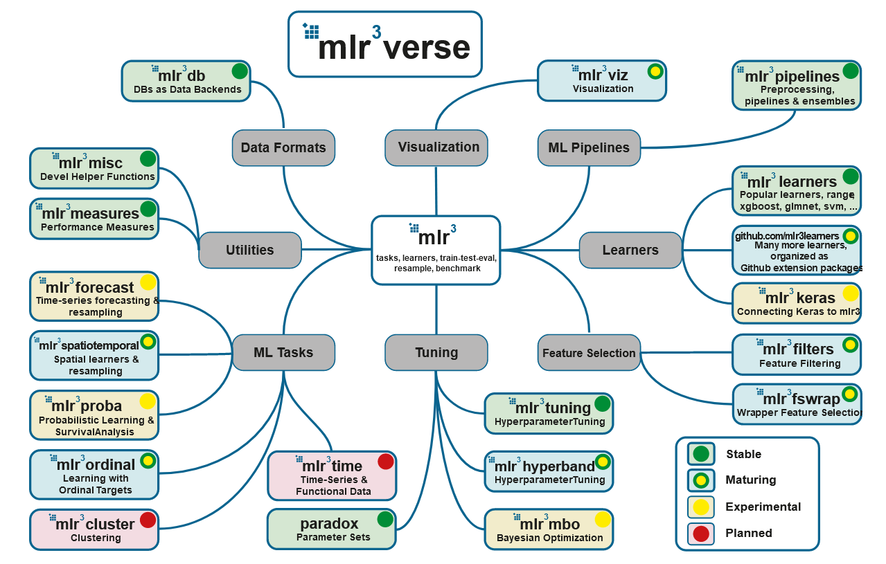
5. mlr3

: mlr3, mlr3tuning paradox. , - mlr3verse:

# install.packages("mlr3verse")
library(mlr3verse)
## Loading required package: mlr3
## Loading required package: mlr3db
## Loading required package: mlr3filters
## Loading required package: mlr3learners
## Loading required package: mlr3pipelines
## Loading required package: mlr3tuning
## Loading required package: mlr3viz
## Loading required package: paradox

mlr3db dbplyr data.table.
mlr3filters , ( ).
mlr3learners (regr.glmnet, regr.kknn, regr.km, regr.lm, regr.ranger, regr.svm, regr.xgboost) (classif.glmnet, classif.kknn, classif.lda, classif.log_reg, classif.multinom, classif.naive_bayes, classif.qda, classif.ranger, classif.svm, classif.xgboost). .
mlr3pipelines (pipelines), . , , CRAN, : remotes::install_github("https://github.com/mlr-org/mlr3pipelines").
mlr3tuning .
mlr3viz , .
mlr3measures — ~40 . mlr3verse , .

, .

6.

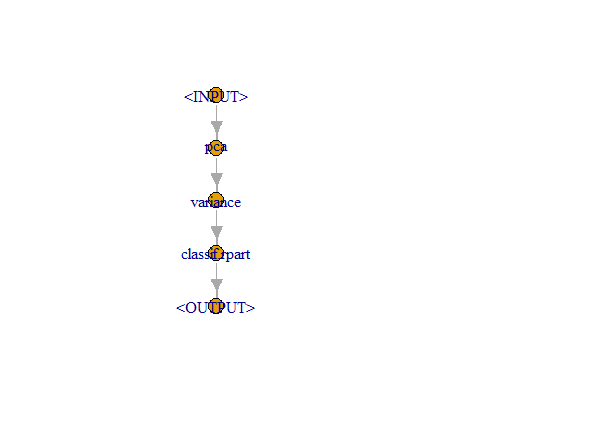
(pipelines) , , .

— , , — . PipeOpLearner(), — PipeOpFilter(), — PipeOp(). ( po()) :

pca <- po("pca")
filter <- po("filter", 
             filter = mlr3filters::flt("variance"), 
             filter.frac = 0.5)
learner_po <- po("learner", 
                 learner = lrn("classif.rpart"))

%>>%:

graph <- pca %>>% filter %>>% learner_po
graph$plot()

. , :

gr <- Graph$new()$
  add_pipeop(mlr_pipeops$get("copy", outnum = 2))$
  add_pipeop(mlr_pipeops$get("scale"))$
  add_pipeop(mlr_pipeops$get("pca"))$
  add_pipeop(mlr_pipeops$get("featureunion", innum = 2))

gr$
  add_edge("copy", "scale", src_channel = 1)$        
  add_edge("copy", "pca", src_channel = "output2")$  
  add_edge("scale", "featureunion", dst_channel = 1)$
  add_edge("pca", "featureunion", dst_channel = 2)

gr$plot(html = FALSE)

, (po("learner", learner = lrn("classif.rpart"))). , :

glrn <- GraphLearner$new(graph)
glrn 
# <GraphLearner:pca.variance.classif.rpart>
# * Model: -
# * Parameters: variance.filter.frac=0.5, variance.na.rm=TRUE, classif.rpart.xval=0
# * Packages: -
# * Predict Type: response
# * Feature types: logical, integer, numeric, character, factor, ordered, POSIXct
# * Properties: importance, missings, multiclass, oob_error, selected_features, twoclass,
#   weights

GraphLearner Learner. , Learner-, :

resample(tsk("iris"), glrn, rsmp("cv"))
# INFO  [17:17:00.358] Applying learner 'pca.variance.classif.rpart' on task 'iris' (iter 1/10) 
# INFO  [17:17:00.615] Applying learner 'pca.variance.classif.rpart' on task 'iris' (iter 2/10) 
# INFO  [17:17:00.881] Applying learner 'pca.variance.classif.rpart' on task 'iris' (iter 3/10) 
# INFO  [17:17:01.087] Applying learner 'pca.variance.classif.rpart' on task 'iris' (iter 4/10) 
# INFO  [17:17:01.303] Applying learner 'pca.variance.classif.rpart' on task 'iris' (iter 5/10) 
# INFO  [17:17:01.518] Applying learner 'pca.variance.classif.rpart' on task 'iris' (iter 6/10) 
# INFO  [17:17:01.716] Applying learner 'pca.variance.classif.rpart' on task 'iris' (iter 7/10) 
# INFO  [17:17:01.927] Applying learner 'pca.variance.classif.rpart' on task 'iris' (iter 8/10) 
# INFO  [17:17:02.129] Applying learner 'pca.variance.classif.rpart' on task 'iris' (iter 9/10) 
# INFO  [17:17:02.337] Applying learner 'pca.variance.classif.rpart' on task 'iris' (iter 10/10) 
# <ResampleResult> of 10 iterations
# * Task: iris
# * Learner: pca.variance.classif.rpart
# * Warnings: 0 in 0 iterations
# * Errors: 0 in 0 iterations

, issue How to deal with different preprocessing steps as hyperparameters:

gr <- pipeline_branch(list(pca = po("pca"), nothing = po("nop")))
gr$plot()

caret tidymodels !

, mlr3. mlr3 book .

Aprendizaje automático en lenguaje R usando el paquete mlr3