Detección de anomalías de Python con codificadores automáticos en Python

La detección de anomalías es una tarea interesante de aprendizaje automático. No hay una forma específica de resolverlo, ya que cada conjunto de datos tiene sus propias características. Pero al mismo tiempo, hay varios enfoques que ayudan a tener éxito. Quiero hablar sobre uno de estos enfoques: autoencoders.

¿Qué conjunto de datos elegir?

El problema más apremiante en la vida de cualquier científico de datos. Para simplificar la historia, usaré un conjunto de datos simple en la estructura, que generaremos aquí.

#  
import os
import numpy as np
from sklearn.model_selection import train_test_split
import matplotlib.pyplot as plt
from matplotlib.colors import Normalize

#        
def gen_normal_distribution(mu, sigma, size, range=(0, 1), max_val=1):
  bins = np.linspace(*range, size)
  result = 1 / (sigma * np.sqrt(2*np.pi)) * np.exp(-(bins - mu)**2 / (2*sigma**2))

  cur_max_val = result.max()
  k = max_val / cur_max_val

  result *= k

  return result

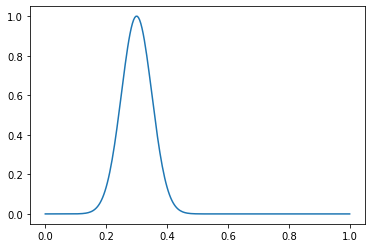
Considere un ejemplo de una función. Cree una distribución normal con μ = 0.3 y σ = 0.05:

dist = gen_normal_distribution(0.3, 0.05, 256, max_val=1)
print(dist.max())
>>> 1.0
plt.plot(np.linspace(0, 1, 256), dist)

Declarar los parámetros de nuestro conjunto de datos:

in_distribution_size = 2000
out_distribution_size = 200
val_size = 100
sample_size = 256

random_generator = np.random.RandomState(seed=42) #    seed

Y las funciones para generar ejemplos son normales y anormales. Las distribuciones con un máximo se considerarán normales, anormales, con dos:

def generate_in_samples(size, sample_size):
  global random_generator

  in_samples = np.zeros((size, sample_size))

  in_mus = random_generator.uniform(0.1, 0.9, size)
  in_sigmas = random_generator.uniform(0.05, 0.5, size)

  for i in range(size):
    in_samples[i] = gen_normal_distribution(in_mus[i], in_sigmas[i], sample_size, max_val=1)

  return in_samples

def generate_out_samples(size, sample_size):
  global random_generator

  #     
  out_samples = generate_in_samples(size, sample_size)

  #        
  out_additional_mus = random_generator.uniform(0.1, 0.9, size)
  out_additional_sigmas = random_generator.uniform(0.01, 0.05, size)

  for i in range(size):
    anomaly = gen_normal_distribution(out_additional_mus[i], out_additional_sigmas[i], sample_size, max_val=0.12)
    out_samples[i] += anomaly

  return out_samples

Así es como se ve un ejemplo normal:

in_samples = generate_in_samples(in_distribution_size, sample_size)
plt.plot(np.linspace(0, 1, sample_size), in_samples[42])

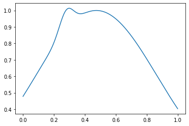
Y anormal, como este:

out_samples = generate_out_samples(out_distribution_size, sample_size)
plt.plot(np.linspace(0, 1, sample_size), out_samples[42])

Crear matrices con etiquetas y etiquetas:

x = np.concatenate((in_samples, out_samples))
#     0,  -- 1
y = np.concatenate((np.zeros(in_distribution_size), np.ones(out_distribution_size)))

#   / 
x_train, x_test, y_train, y_test = train_test_split(x, y, test_size=0.2, shuffle=True, random_state=42)

. , , 2 1 (). , ( ), :

#     100   100  
x_val_out = generate_out_samples(val_size, sample_size)
x_val_in = generate_in_samples(val_size, sample_size)

x_val = np.concatenate((x_val_out, x_val_in))
y_val = np.concatenate((np.ones(val_size), np.zeros(val_size)))

, , Sklearn: SVM . , , .

#     
from sklearn.metrics import classification_report
from sklearn.metrics import f1_score

One class SVM

from sklearn.svm import OneClassSVM

OneClassSVM nu — .

out_dist_part = out_distribution_size / (out_distribution_size + in_distribution_size)
svm = OneClassSVM(nu=out_dist_part)
svm.fit(x_train, y_train)
>>> OneClassSVM(cache_size=200, coef0=0.0, degree=3, gamma='scale', kernel='rbf',
            max_iter=-1, nu=0.09090909090909091, shrinking=True, tol=0.001,
            verbose=False)

:

svm_prediction = svm.predict(x_val)
svm_prediction[svm_prediction == 1] = 0
svm_prediction[svm_prediction == -1] = 1

sklearn — classification_report, Anomaly detection , precision recall, :

print(classification_report(y_val, svm_prediction))

>>>           precision    recall  f1-score   support

         0.0       0.57      0.93      0.70       100
         1.0       0.81      0.29      0.43       100

    accuracy                           0.61       200
   macro avg       0.69      0.61      0.57       200
weighted avg       0.69      0.61      0.57       200

, . f1-score , .

Isolation forest

, , - ?

from sklearn.ensemble import IsolationForest

, . :

out_dist_part = out_distribution_size / (out_distribution_size + in_distribution_size)

iso_forest = IsolationForest(n_estimators=100, contamination=out_dist_part, max_features=100, n_jobs=-1)
iso_forest.fit(x_train)
>>> IsolationForest(behaviour='deprecated', bootstrap=False,
                contamination=0.09090909090909091, max_features=100,
                max_samples='auto', n_estimators=100, n_jobs=-1,
                random_state=None, verbose=0, warm_start=False)

Classification report? — Classification report!

iso_forest_prediction = iso_forest.predict(x_val)
iso_forest_prediction[iso_forest_prediction == 1] = 0
iso_forest_prediction[iso_forest_prediction == -1] = 1

print(classification_report(y_val, iso_forest_prediction))
>>>            precision    recall  f1-score   support

         0.0       0.50      0.91      0.65       100
         1.0       0.53      0.10      0.17       100

    accuracy                           0.51       200
   macro avg       0.51      0.51      0.41       200
weighted avg       0.51      0.51      0.41       200

RandomForestClassifier

, - " ?" , :

from sklearn.ensemble import RandomForestClassifier

random_forest = RandomForestClassifier(n_estimators=100, max_features=100, n_jobs=-1)
random_forest.fit(x_train, y_train)
>>> RandomForestClassifier(bootstrap=True, ccp_alpha=0.0, class_weight=None,
                       criterion='gini', max_depth=None, max_features=100,
                       max_leaf_nodes=None, max_samples=None,
                       min_impurity_decrease=0.0, min_impurity_split=None,
                       min_samples_leaf=1, min_samples_split=2,
                       min_weight_fraction_leaf=0.0, n_estimators=100,
                       n_jobs=-1, oob_score=False, random_state=None, verbose=0,
                       warm_start=False)

random_forest_prediction = random_forest.predict(x_val)
print(classification_report(y_val, random_forest_prediction))
>>>            precision    recall  f1-score   support

         0.0       0.57      0.99      0.72       100
         1.0       0.96      0.25      0.40       100

    accuracy                           0.62       200
   macro avg       0.77      0.62      0.56       200
weighted avg       0.77      0.62      0.56       200

Autoencoder

, : . .

, "" , . 2 : Encoder' Decoder', .

"" , , .

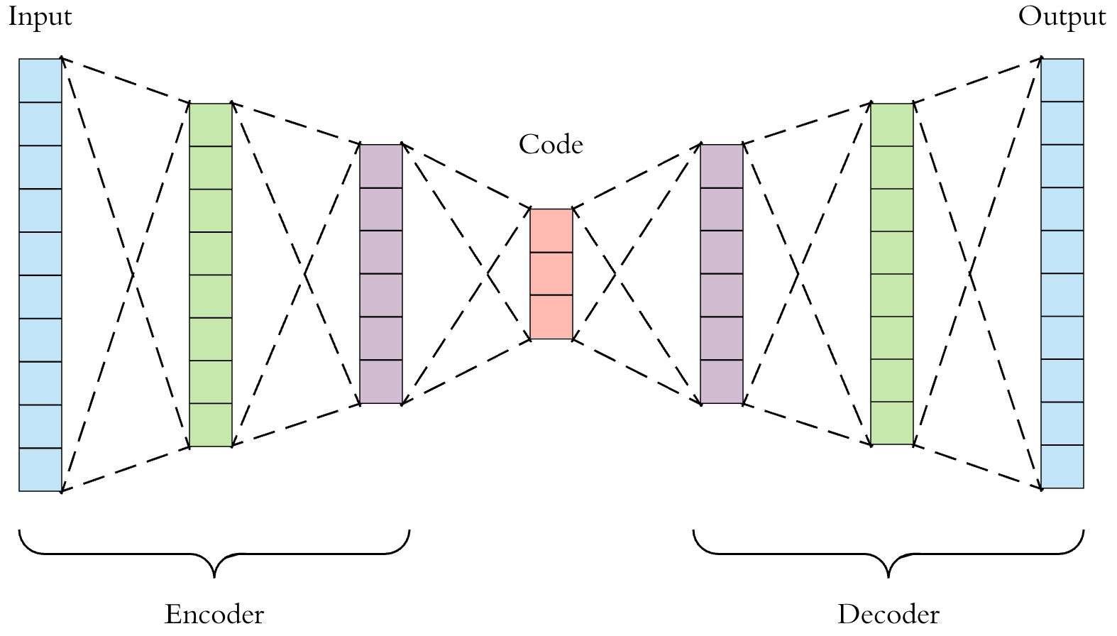
? , , , . , 9% 91% . , . , , : .

.

PyTorch, :

import torch
from torch import nn
from torch.utils.data import TensorDataset, DataLoader
from torch.optim import Adam

:

batch_size = 32
lr = 1e-3

. , , "" . , ( , learning rate, ) , , .

#      x_train,    
train_in_distribution = x_train[y_train == 0]
train_in_distribution = torch.tensor(train_in_distribution.astype(np.float32))

train_in_dataset = TensorDataset(train_in_distribution)
train_in_loader = DataLoader(train_in_dataset, batch_size=batch_size, shuffle=True)

#       ,           
test_dataset = TensorDataset(
    torch.tensor(x_test.astype(np.float32)),
    torch.tensor(y_test.astype(np.long))
)
test_loader = DataLoader(test_dataset, batch_size=batch_size, shuffle=False)

val_dataset = TensorDataset(torch.tensor(x_val.astype(np.float32)))
val_loader = DataLoader(val_dataset, batch_size=batch_size, shuffle=False)

. 4 , ( 2 : μ, — σ, ; 4 , ).

class Autoencoder(nn.Module):
  def __init__(self, input_size):
    super(Autoencoder, self).__init__()
    self.encoder = nn.Sequential(
      nn.Linear(input_size, 128),
      nn.LeakyReLU(0.2),
      nn.Linear(128, 64),
      nn.LeakyReLU(0.2),
      nn.Linear(64, 16),
      nn.LeakyReLU(0.2),
      nn.Linear(16, 4),
      nn.LeakyReLU(0.2),
    )
    self.decoder = nn.Sequential(
      nn.Linear(4, 16),
      nn.LeakyReLU(0.2),
      nn.Linear(16, 64),
      nn.LeakyReLU(0.2),
      nn.Linear(64, 128),
      nn.LeakyReLU(0.2),
      nn.Linear(128, 256),
      nn.LeakyReLU(0.2),
    )

  def forward(self, x):
    x = self.encoder(x)
    x = self.decoder(x)
    return x

model = Autoencoder(sample_size).cuda()
criterion = nn.MSELoss()
per_sample_criterion = nn.MSELoss(reduction="none") # loss   ,   
#   reduction="none" pytorch  loss'   
optimizer = Adam(model.parameters(), lr=lr, weight_decay=1e-5)

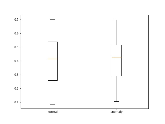
- loss' , , boxplot' :

def save_score_distribution(model, data_loader, criterion, save_to, figsize=(8, 6)):
  losses = [] #    loss    
  labels = [] #  --  
  for (x_batch, y_batch) in data_loader:
    x_batch = x_batch.cuda()

    output = model(x_batch)
    loss = criterion(output, x_batch)

    loss = torch.mean(loss, dim=1) #  loss    (        )
    loss = loss.detach().cpu().numpy().flatten()
    losses.append(loss)

    labels.append(y_batch.detach().cpu().numpy().flatten())

  losses = np.concatenate(losses)
  labels = np.concatenate(labels)

  losses_0 = losses[labels == 0] #  
  losses_1 = losses[labels == 1] #  

  fig, ax = plt.subplots(1, figsize=figsize)

  ax.boxplot([losses_0, losses_1])
  ax.set_xticklabels(['normal', 'anomaly'])

  plt.savefig(save_to)
  plt.close(fig)

:

:

experiment_path = "ood_detection" #    
!rm -rf $experiment_path
os.makedirs(experiment_path, exist_ok=True)

epochs = 100

for epoch in range(epochs):
  running_loss = 0
  for (x_batch, ) in train_in_loader:
    x_batch = x_batch.cuda()

    output = model(x_batch)
    loss = criterion(output, x_batch)

    optimizer.zero_grad()
    loss.backward()
    optimizer.step()

    running_loss += loss.item()

  print("epoch [{}/{}], train loss:{:.4f}".format(epoch+1, epochs, running_loss))

  #   
  plot_path = os.path.join(experiment_path, "{}.jpg".format(epoch+1))
  save_score_distribution(model, test_loader, per_sample_criterion, plot_path)

>>> 
epoch [1/100], train loss:8.5728
epoch [2/100], train loss:4.2405
epoch [3/100], train loss:4.0852
epoch [4/100], train loss:1.7578
epoch [5/100], train loss:0.8543
...
epoch [96/100], train loss:0.0147
epoch [97/100], train loss:0.0154
epoch [98/100], train loss:0.0117
epoch [99/100], train loss:0.0105
epoch [100/100], train loss:0.0097

50

100

, . , :

# ,    
def get_prediction(model, x):
  global batch_size

  dataset = TensorDataset(torch.tensor(x.astype(np.float32)))
  data_loader = DataLoader(dataset, batch_size=batch_size, shuffle=False)

  predictions = []
  for batch in data_loader:
    x_batch = batch[0].cuda()
    pred = model(x_batch) # x -> encoder -> decoder -> x_pred
    predictions.append(pred.detach().cpu().numpy())

  predictions = np.concatenate(predictions)
  return predictions

#      (  )
def compare_data(xs, sample_num, data_range=(0, 1), labels=None):
  fig, axes = plt.subplots(len(xs))
  sample_size = len(xs[0][sample_num])

  for i in range(len(xs)):
    axes[i].plot(np.linspace(*data_range, sample_size), xs[i][sample_num])

  if labels:
    for i, label in enumerate(labels):
      axes[i].set_ylabel(label)

:

x_test_pred = get_prediction(model, x_test)
compare_data([x_test[y_test == 0], x_test_pred[y_test == 0]], 10, labels=["real", "encoded"])

:

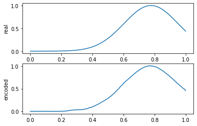
X? .

Difference score

— . , , , . .

def get_difference_score(model, x):
  global batch_size

  dataset = TensorDataset(torch.tensor(x.astype(np.float32)))
  data_loader = DataLoader(dataset, batch_size=batch_size, shuffle=False)

  predictions = []
  for (x_batch, ) in data_loader:
    x_batch = x_batch.cuda()
    preds = model(x_batch)
    predictions.append(preds.detach().cpu().numpy())

  predictions = np.concatenate(predictions)

  #     
  return (x - predictions)

from sklearn.ensemble import RandomForestClassifier

test_score = get_difference_score(model, x_test)

score_forest = RandomForestClassifier(max_features=100)
score_forest.fit(test_score, y_test)
>>> RandomForestClassifier(bootstrap=True, ccp_alpha=0.0, class_weight=None,
                       criterion='gini', max_depth=None, max_features=100,
                       max_leaf_nodes=None, max_samples=None,
                       min_impurity_decrease=0.0, min_impurity_split=None,
                       min_samples_leaf=1, min_samples_split=2,
                       min_weight_fraction_leaf=0.0, n_estimators=100,
                       n_jobs=None, oob_score=False, random_state=None,
                       verbose=0, warm_start=False)

, : 2 — . , 2 : , — difference_score, — . , , .

? . difference_score , ( ) , , . , , difference_score , ( ). .

:

val_score = get_difference_score(model, x_val)
prediction = score_forest.predict(val_score)
print(classification_report(y_val, prediction))
>>>            precision    recall  f1-score   support

         0.0       0.76      1.00      0.87       100
         1.0       1.00      0.69      0.82       100

    accuracy                           0.84       200
   macro avg       0.88      0.84      0.84       200
weighted avg       0.88      0.84      0.84       200

. :

indices = np.arange(len(prediction))
#       ,     
wrong_indices = indices[(prediction == 0) & (y_val == 1)]

x_val_pred = get_prediction(model, x_val)
compare_data([x_val, x_val_pred], wrong_indices[0])

? :

plt.imshow(val_score[wrong_indices], norm=Normalize(0, 1, clip=True))

:

plt.imshow(val_score[(prediction == 1) & (y_val == 1)], norm=Normalize(0, 1, clip=True))

:

plt.imshow(val_score[(prediction == 0) & (y_val == 0)], norm=Normalize(0, 1, clip=True))

, : .

Difference histograms

. . — , "", .

, difference score

print("test score: [{}; {}]".format(test_score.min(), test_score.max()))
>>> test score: [-0.2260764424351479; 0.26339245919832344]

, :

def score_to_histograms(scores, bins=10, data_range=(-0.3, 0.3)):
  result_histograms = np.zeros((len(scores), bins))

  for i in range(len(scores)):
    hist, bins = np.histogram(scores[i], bins=bins, range=data_range)
    result_histograms[i] = hist

  return result_histograms

test_histogram = score_to_histograms(test_score, bins=10, data_range=(-0.3, 0.3))
val_histogram = score_to_histograms(val_score, bins=10, data_range=(-0.3, 0.3))

plt.title("normal histogram")
plt.bar(np.linspace(-0.3, 0.3, 10), test_histogram[y_test == 0][0])

plt.title("anomaly histogram")
plt.bar(np.linspace(-0.3, 0.3, 10), test_histogram[y_test == 1][0])

, "", .

histogram_forest = RandomForestClassifier(n_estimators=10)
histogram_forest.fit(test_histogram, y_test)
>>> RandomForestClassifier(bootstrap=True, ccp_alpha=0.0, class_weight=None,
                       criterion='gini', max_depth=None, max_features='auto',
                       max_leaf_nodes=None, max_samples=None,
                       min_impurity_decrease=0.0, min_impurity_split=None,
                       min_samples_leaf=1, min_samples_split=2,
                       min_weight_fraction_leaf=0.0, n_estimators=10,
                       n_jobs=None, oob_score=False, random_state=None,
                       verbose=0, warm_start=False)

val_prediction = histogram_forest.predict(val_histogram)
print(classification_report(y_val, val_prediction))
>>>            precision    recall  f1-score   support

         0.0       0.83      0.99      0.90       100
         1.0       0.99      0.80      0.88       100

    accuracy                           0.90       200
   macro avg       0.91      0.90      0.89       200
weighted avg       0.91      0.90      0.89       200

— . , , , , . () .

— . ? VAE, ( 4 ) . . CVAE, - . , , , ..

GAN', (), . ( ).

, , .

, Data science' . Computer vision, . ( — !) — FARADAY Lab. — , .

c:

• Detección de anomalías en el análisis de imágenes médicas
• Detección de anomalías para dummies.
• Métodos de detección de anomalías
• Mejorando la detección de OOD