Hello, Habr! Today I want to share a small example of how to conduct cluster analysis. In this example, the reader will not find neural networks and other fashionable directions. This example can serve as a reference point in order to make a small and complete cluster analysis for other data. Anyone interested - welcome to cat.
Immediately make a reservation, this article in no way claims to be academic in its entirety, uniqueness of the results obtained, or completeness of coverage of the issue. The article is intended to demonstrate the basic steps of classical cluster analysis, which can be used for simple and meaningful (possibly preceding a more detailed) study. Any corrections, comments and additions on the merits are welcome.
The data is a sample of alcohol consumption by country per capita by type of alcoholic beverages (beer, wine, spirits, etc.) for 2010 as a percentage of per capita alcohol consumption. The data also contains: average daily alcohol consumption per capita in grams of pure alcohol and all (recorded + unaccounted) alcohol consumption per capita (only drinkers in liters of pure alcohol).
At the same time, each country conditionally belongs to one of the geographical groups: east, center and west. The division is very arbitrary and very controversial for various reasons, but we will proceed from what we have. Data Source - Global status report on alcohol and health 2014, S. 289-364
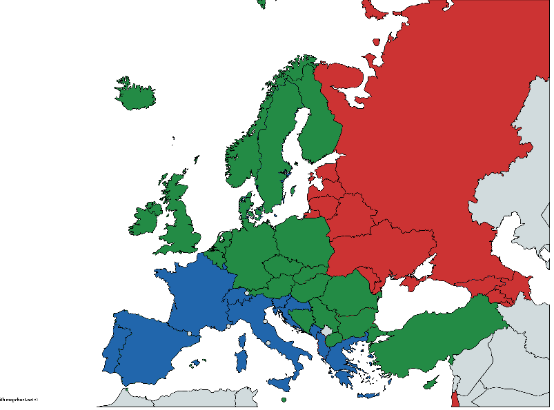
(Hand-painted, there may be errors, but the general idea, I think, is understandable)
Preliminary analysis
Connect the libraries used.
library(rgl)
library(heplots)
library(MVN)
library(klaR)
library('Morpho')
library(caret)
library(mclust)
library(ggplot2)
library(GGally)
library(plyr)
library(psych)
library(GPArotation)
library(ggpubr)
, .
#
data <- read.table("alcohol_data.csv", header=TRUE,  sep=",")
#
rownames(data) <- make.names(data[,1], unique = TRUE)
#     ,
data <- data[,-1]
data <- na.omit(data)
#
head(data)
summary(data)
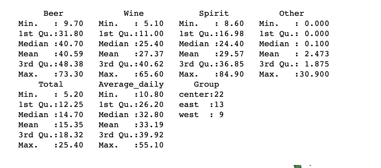
, . , Other , , , , . , , , , . , . - .
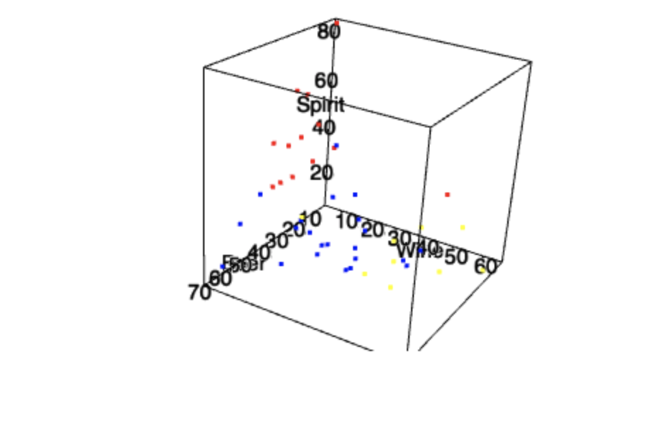
, , , .
options(rgl.useNULL=TRUE)
open3d()
mfrow3d(2,2)
levelColors <- c('west'='blue', 'east'='red', 'center'='yellow')
plot3d(data$Beer, data$Wine, data$Spirit, xlab="Beer", ylab="Wine", zlab="Spirit", col = levelColors[data$Group], size=3)

widget <- rglwidget()
widget
, . , .
ggpairs(
  data,
  mapping = ggplot2::aes(color = data$Group),
  upper = list(continuous = wrap("cor", alpha = 0.5), combo = "box"),
  lower = list(continuous = wrap("points", alpha = 0.3), combo = wrap("dot", alpha = 0.4)),
  diag = list(continuous = wrap("densityDiag",alpha = 0.5)),
  title = "Alcohol"
)
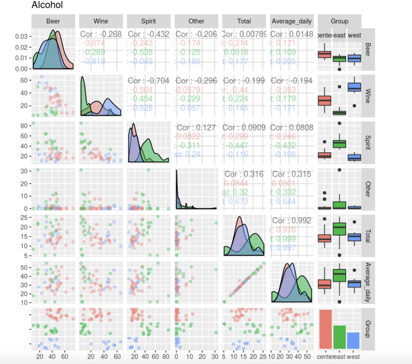
Average Total , Average.
data <- data[, -6]
, , , , . .
data[data$Wine>60,]
, , , , - , , .
data[data$Spirit>70,]
data[data$Spirit<10,]
, , .
,
split(data[,1:5],data$Group)
$center
$east
$west
ggpairs(
  data,
  mapping = ggplot2::aes(color = data$Group),
  diag=list(continuous="bar", alpha=0.4)
)
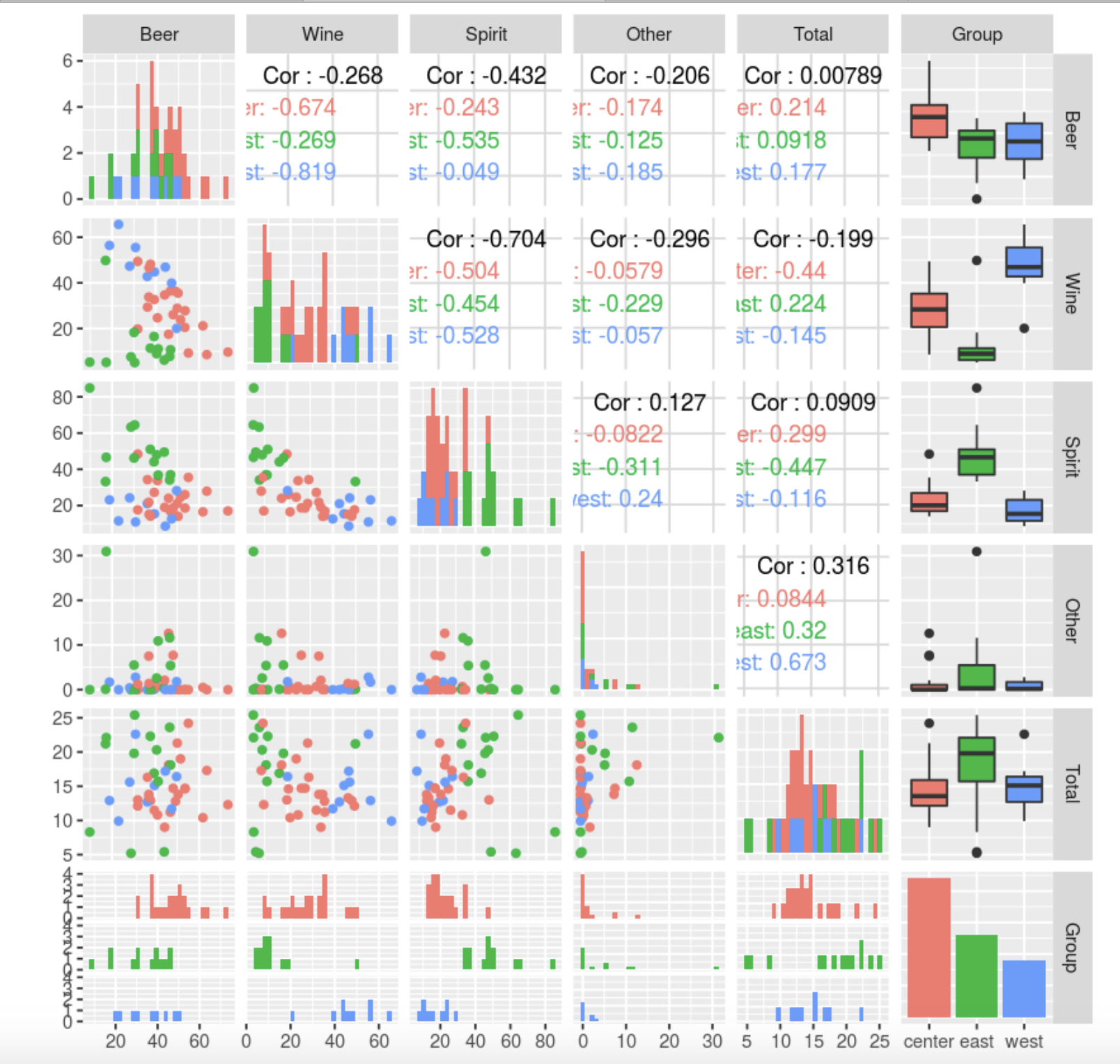
, , . Other, : , , , ( 10-12 , 45, , ). . , , , (). , , . Other .
, , — , — . , — , .
Total Other, . .
, Beer, Spirit Wine . , , , . , , , , , .
Total. , — .
data.group = data[,5]
data <- data[,-5]
data<- data[,-4]
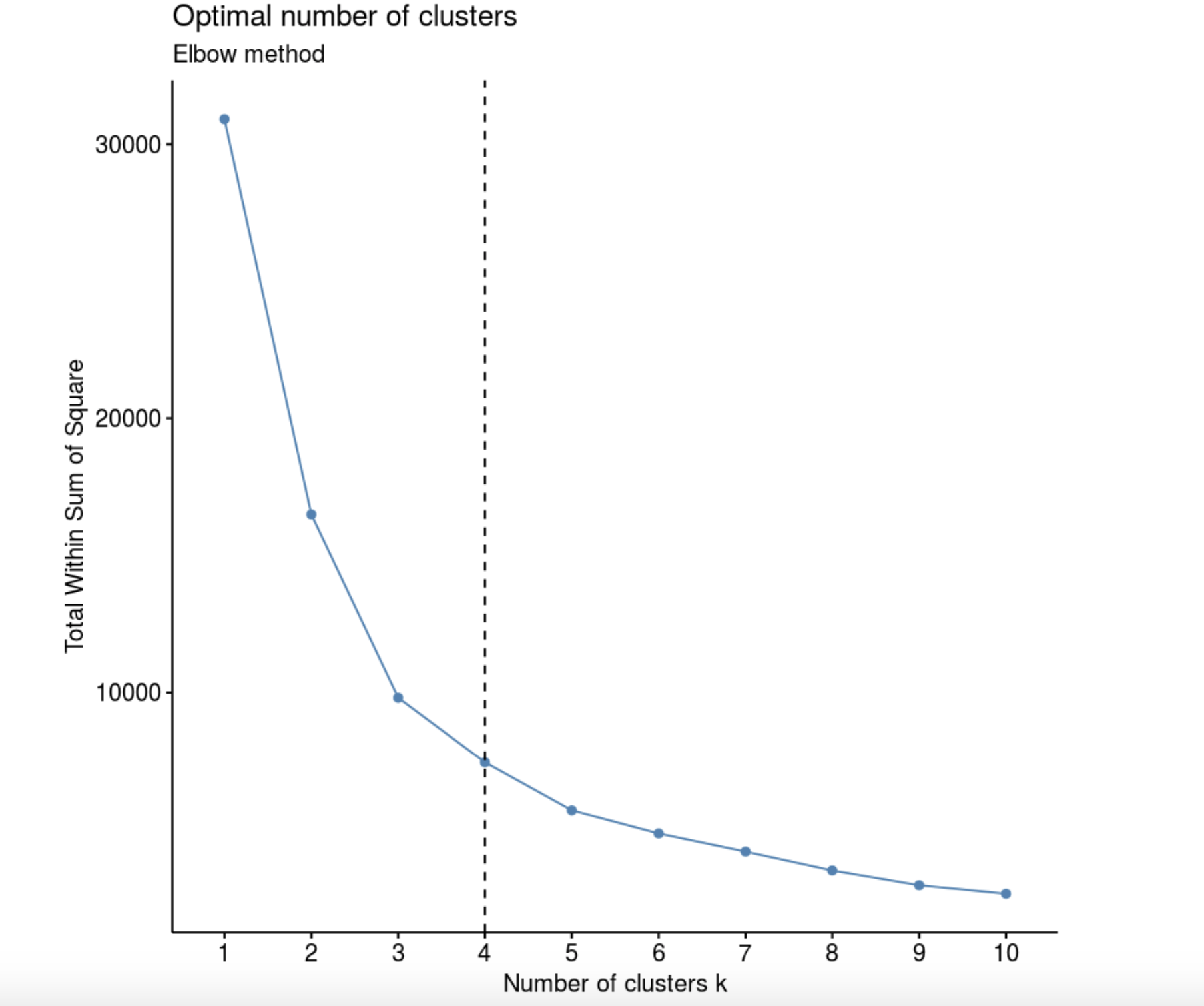
Elbow method (“ ”, “ ”). , k, – W(K), .
library(factoextra)
fviz_nbclust(data, kmeans, method = "wss") +
  labs(subtitle = "Elbow method") +
  geom_vline(xintercept = 4, linetype = 2)
data.dist <- dist((data))
hc <- hclust(data.dist, method = "ward.D2")
plot(hc, cex = 0.7)
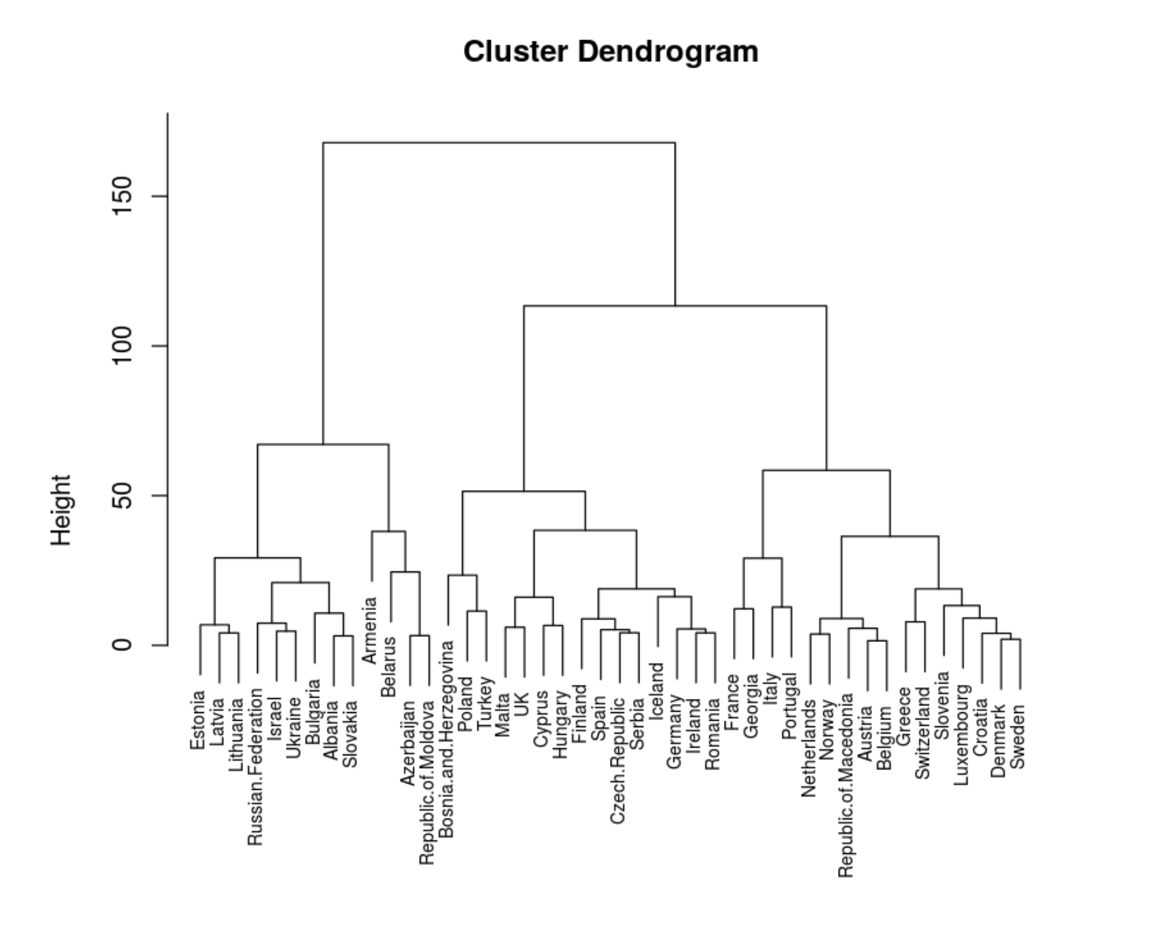
. .
colors=c('green', 'red', 'blue')
hcd = as.dendrogram(hc)
clusMember = cutree(hc, 4)
colLab <- function(n) {
    if (is.leaf(n)) {
        a <- attributes(n)
        labCol <- colors[data.group[n]]
        attr(n, "nodePar") <- c(a$nodePar, lab.col = labCol)
    }
    n
}
clusDendro = dendrapply(hcd, colLab)
plot(clusDendro, main = "Cool Dendrogram", type = "triangle")

rect.hclust(hc, k = 4)
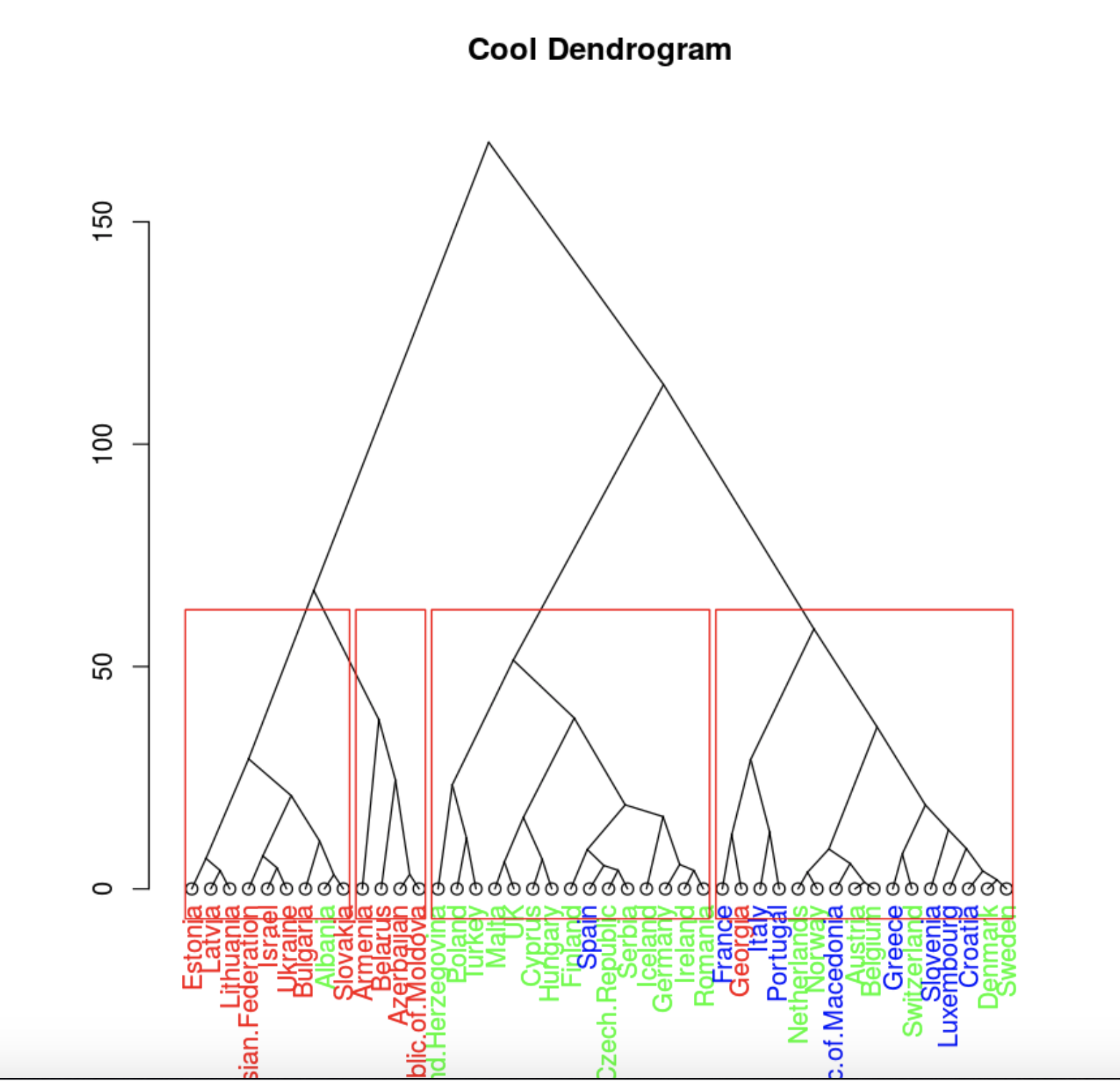
. , .
, , , 4 .
plot(clusDendro, main = "Cool Dendrogram", type = "triangle")
data.hclas_group <- factor(cutree(hc, k = 3))

rect.hclust(hc, k = 3)
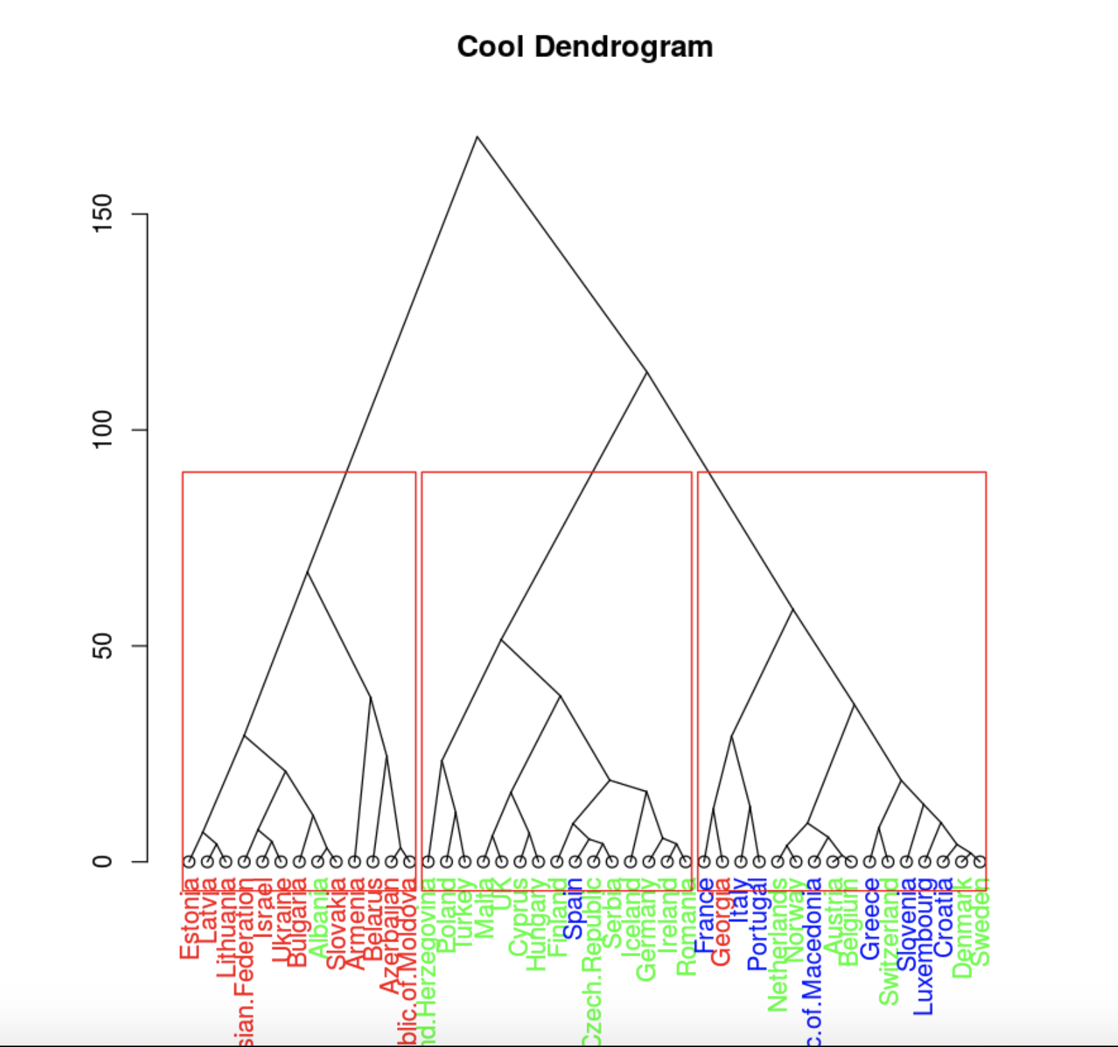
, , .
library(FactoMineR)
res.pca <- PCA(data,scale.unit=T, graph = F)
fviz_pca_biplot(res.pca,
                col = colors[data.hclas_group], palette = "jco",
                label = "var",
                ellipse.level = 0.8,
                 addEllipses = T,
                col.var = "black",
                legend.title = "groups4")
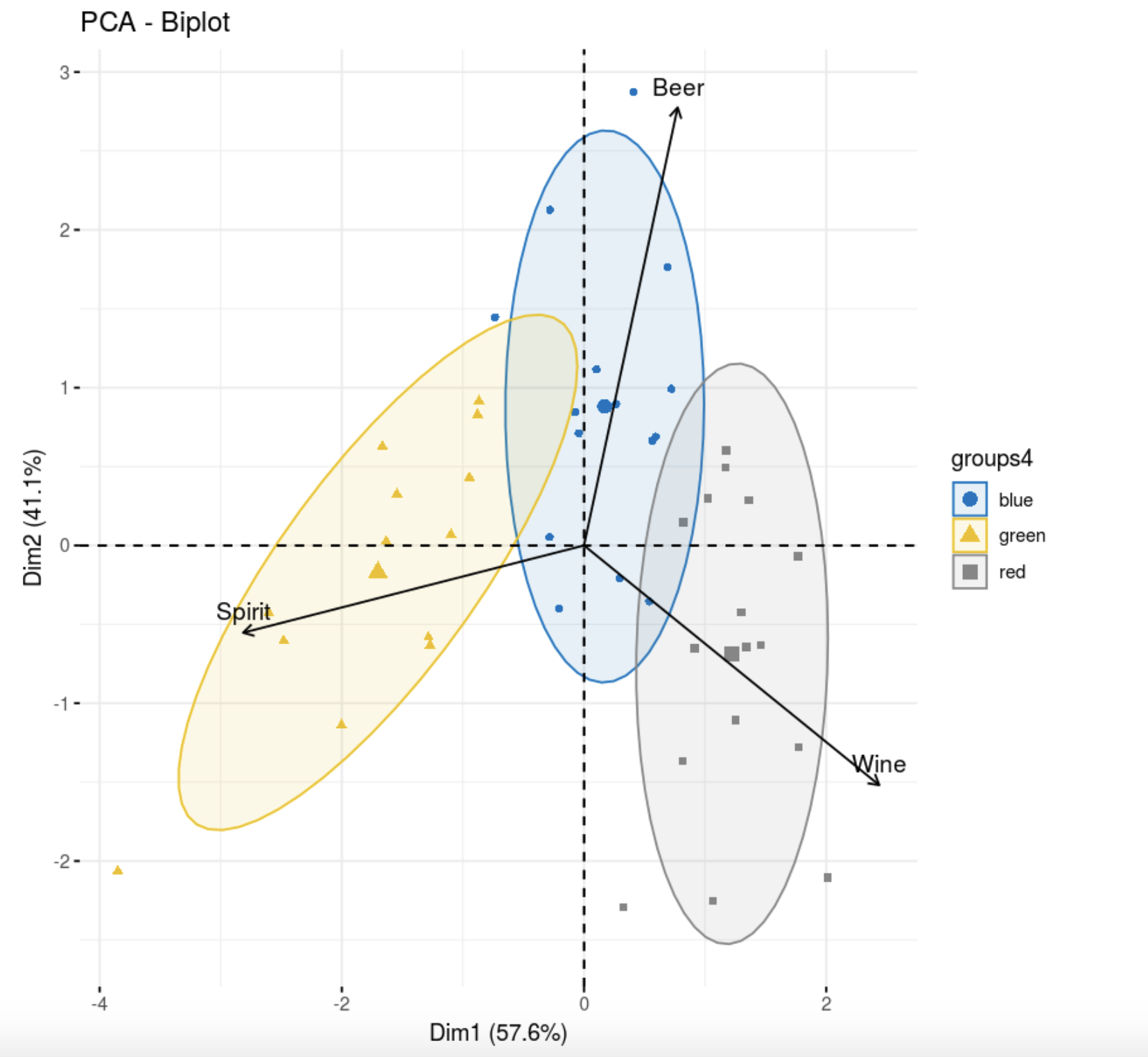
, , . , , , , . , , , k-++.
library(flexclust)
data.kk <- kcca(data, k=3, family=kccaFamily("kmeans"),
control=list(initcent="kmeanspp"))

fviz_pca_biplot(res.pca,
                col.ind =as.factor(data.kk@cluster), palette = "jco",
                label = "var",
                ellipse.level = 0.8,
                 addEllipses = T,
                col.var = "black", repel = TRUE,
                legend.title = "clusters")
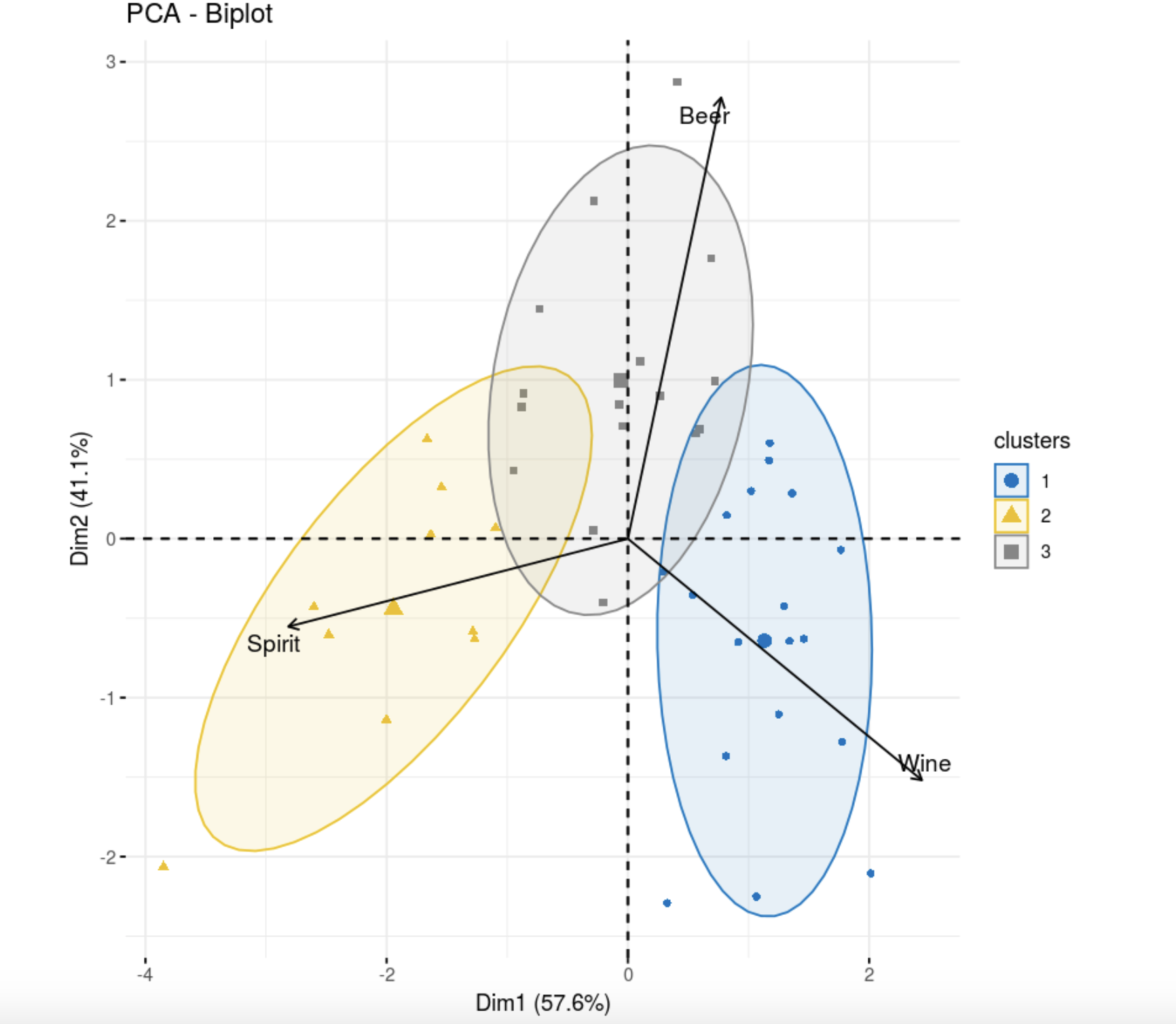
, k- . , , .
, , hclust. .
, , . . , .
. . , , , . , , . , .
It would be possible to carry out clustering based on the assumption of cluster models using information criteria ( here is the description ), as well as try the classical discriminant analysis for this data set. If this article was useful, I plan to publish a sequel.