🚮 👩‍✈️ 👨🏻‍💻 What we pay attention to when calculating the statistical significance of the A / B test 🐬 🏺 🍋

In Uchi.ru, we try to roll out even small improvements with the A / B test, there were more than 250 of them during this academic year. The A / B test is a powerful change testing tool, without which it is difficult to imagine the normal development of an Internet product. At the same time, despite the apparent simplicity, serious errors can be made during the A / B test both at the design stage of the experiment and in summing up the results. In this article I will talk about some of the technical aspects of the test: how we determine the test period, summarize and how to avoid erroneous results when the tests are completed ahead of schedule and when testing several hypotheses at once.

A typical A / B testing scheme for us (and for many) looks like this:

We are developing a feature, but before rolling it out to the entire audience, we want to make sure that it improves the target metric, for example, engagement.
We determine the period for which the test is launched.
We randomly divide users into two groups.
We show one group the product version with features (experimental group), the other - the old one (control).
In the process, we monitor the metric in order to stop a particularly unsuccessful test in time.
After the test expires, we compare the metric in the experimental and control groups.
If the metric in the experimental group is statistically significantly better than in the control group, we roll out the tested feature at all. If there is no statistical significance, we end the test with a negative result.

Everything looks logical and simple, the devil, as always, in the details.

Statistical significance, criteria and errors

There is an element of randomness in any A / B test: group metrics depend not only on their functionality, but also on what users got into them and how they behave. To reliably draw conclusions about the superiority of a group, you need to collect enough observations in the test, but even then you are not immune from mistakes. They are distinguished by two types:

A mistake of the first kind occurs if we fix the difference between the groups, although in reality it does not exist. The text will also contain an equivalent term - a false positive result. The article is devoted to just such errors.
A mistake of the second kind occurs if we fix the absence of a difference, although in fact it is.

With a large number of experiments, it is important that the probability of an error of the first kind is small. It can be controlled using statistical methods. For example, we want the probability of an error of the first kind in each experiment not to exceed 5% (this is just a convenient value, you can take another for your own needs). Then we will take experiments at a significance level of 0.05:

There is an A / B test with control group A and experimental group B. The goal is to verify that group B differs from group A in some metric.
We formulate the null statistical hypothesis: groups A and B do not differ, and the observed differences are explained by noise. By default, we always think that there is no difference until the contrary is proved.
We check the hypothesis with a strict mathematical rule - a statistical criterion, for example, student's criterion.
As a result, we get the p-value. It lies in the range from 0 to 1 and means the probability of seeing the current or more extreme difference between groups, provided that the null hypothesis is true, that is, in the absence of a difference between the groups.
The p-value is compared with a significance level of 0.05. If it is larger, we accept the null hypothesis that there are no differences, otherwise we believe that there is a statistically significant difference between the groups.

A hypothesis can be tested with a parametric or nonparametric criterion. The parametric ones rely on the parameters of the sample distribution of a random variable and have more power (they make mistakes of the second kind less often), but they impose requirements on the distribution of the random variable under study.

The most common parametric test is Student's test. For two independent samples (A / B test case), it is sometimes called the Welch criterion. This criterion works correctly if the studied quantities are distributed normally. It may seem that on real data this requirement is almost never satisfied, but in fact the test requires a normal distribution of sample averages, not the samples themselves. In practice, this means that the criterion can be applied if you have a lot of observations in your test (tens to hundreds) and there are no very long tails in the distributions. The nature of the distribution of the initial observations is unimportant. The reader can independently verify that the Student criterion works correctly even on samples generated from Bernoulli or exponential distributions.

Of the nonparametric criteria, the Mann-Whitney criterion is popular. It should be used if your samples are very small or have large outliers (the method compares the medians, therefore it is resistant to outliers). Also, for the criterion to work correctly, the samples should have few matching values. In practice, we never had to apply nonparametric criteria, in our tests we always use the student criterion.

The problem of multiple hypothesis testing

The most obvious and simplest problem: if in the test, in addition to the control group, there are several experimental ones, then summing up the results with a significance level of 0.05 will lead to a multiple increase in the proportion of errors of the first kind. This happens because with each application of the statistical criterion, the probability of an error of the first kind will be 5%. With the number of groups

n g r o u p s

$ngroups$ and significance level

α

$\alpha$ the probability that some experimental group will win by chance is:

P (a n y f a l s e p o s i t i v e) = 1 - (1 - α)^{n g r o u p s}

$P(any\ false\ positive) = 1 − (1 − \alpha) ^ {ngroups}$

For example, for the three experimental groups we get 14.3% instead of the expected 5%. The problem is solved by Bonferroni's correction for multiple hypothesis testing: you just need to divide the significance level by the number of comparisons (i.e. groups) and work with it. For the example above, the significance level, taking into account the amendment, will be 0.05 / 3 = 0.0167 and the probability of at least one error of the first kind will be acceptable 4.9%.

Hill Method - Bonferroni

— , , , .

n g r o u p s

$ngroups$ p-value ,

s t e p_n u m b e r

$step\_number$ :

α_{s t e p} = \frac{α}{n g r o u p s - s t e p_n u m b e r + 1}

$\alpha_{step} = \frac {\alpha} {ngroups − step\_number + 1}$

P-value

α / n g r o u p s

$\alpha/ngroups$ . , p-value

α / (n g r o u p s - 1)

$\alpha/(ngroups − 1)$ , . - , . ( , ) p-value, . A/B- — , — .

Strictly speaking, comparisons of groups by different metrics or sections of the audience are also subject to the problem of multiple testing. Formally, it’s quite difficult to take into account all the checks, because their number is difficult to predict in advance and sometimes they are not independent (especially when it comes to different metrics, not slices). There is no universal recipe, rely on common sense and remember that if you check a lot of slices using different metrics, then in any test you can see an allegedly statistically significant result. So, one should be careful, for example, to the significant increase in retention of the fifth day of new mobile users from large cities.

Peeping problem

A particular case of multiple hypothesis testing is the peeking problem. The point is that the p-value during the test can accidentally fall below the accepted significance level. If you carefully monitor the experiment, you can catch this moment and make a mistake about the statistical significance.

Suppose we moved away from the test setup described at the beginning of the post and decided to take stock at a significance level of 5% every day (or just more than once during the test). By summing up, I understand that the test is positive if p-value is below 0.05, and its continuation otherwise. With this strategy, the share of false-positive results will be proportional to the number of checks and in the first month will reach 28%. Such a huge difference seems counterintuitive, therefore we turn to the methodology of A / A tests, which is indispensable for the development of A / B testing schemes.

The idea of an A / A test is simple: to simulate a lot of A / B tests on random data with random grouping. There is obviously no difference between the groups, so you can accurately estimate the proportion of errors of the first kind in your A / B testing scheme. The gif below shows how the p-value changes by day for four such tests. An equal 0.05 significance level is indicated by a dashed line. When the p-value falls below, we color the test plot in red. If at this time the results of the test were summed up, it would be considered successful.

Similarly, we calculate 10 thousand A / A-tests lasting one month and compare the fractions of false-positive results in the scheme with summing up at the end of the term and every day. For clarity, here are the p-value wandering schedules by day for the first 100 simulations. Each line is the p-value of one test, the trajectories of the tests are highlighted in red, which are ultimately mistakenly considered successful (the smaller the better), the dashed line is the required p-value to recognize the test as successful.

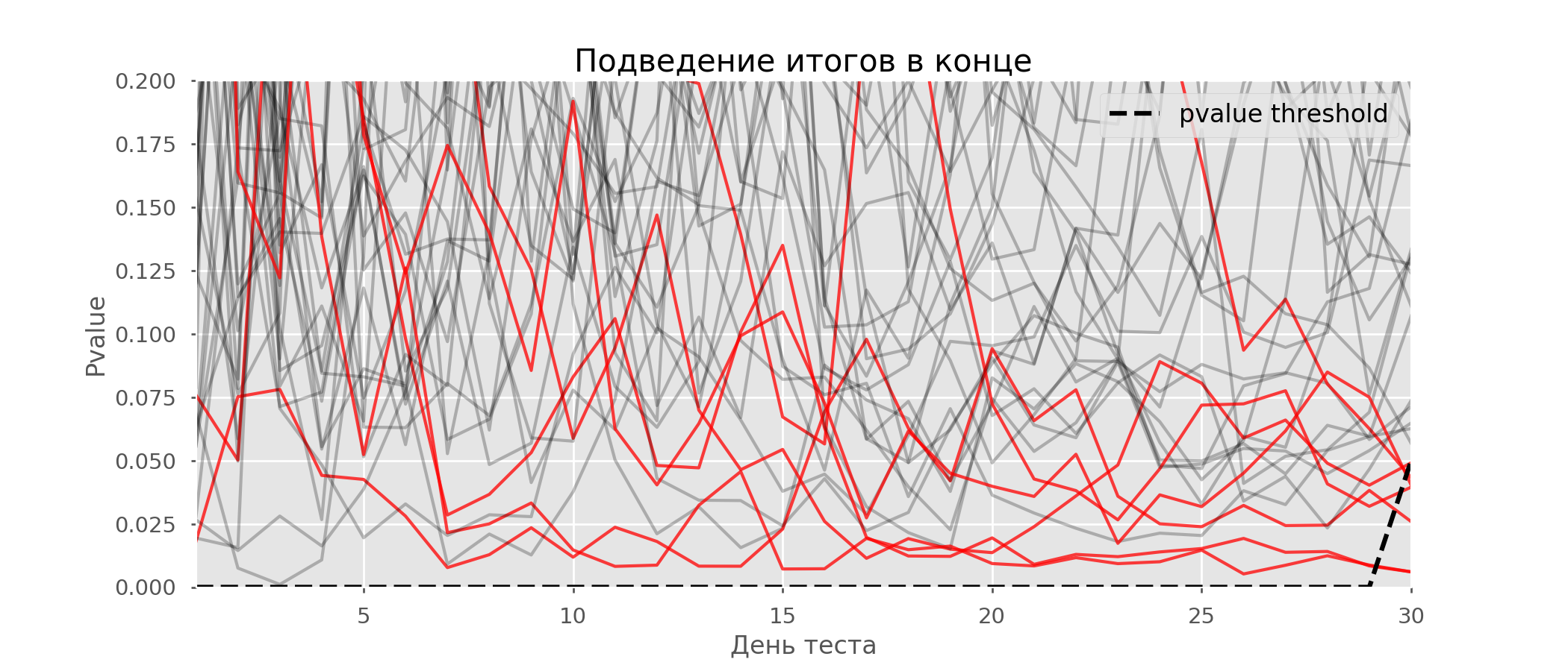On the graph, you can count 7 false-positive tests, and in total among 10 thousand there were 502, or 5%. It should be noted that the p-value of many tests during the course of observations fell below 0.05, but by the end of the observations went beyond the significance level. Now let's evaluate the testing scheme with a debriefing every day:

There are so many red lines that nothing is clear. We will redraw by breaking the test lines as soon as their p-value reaches a critical value:

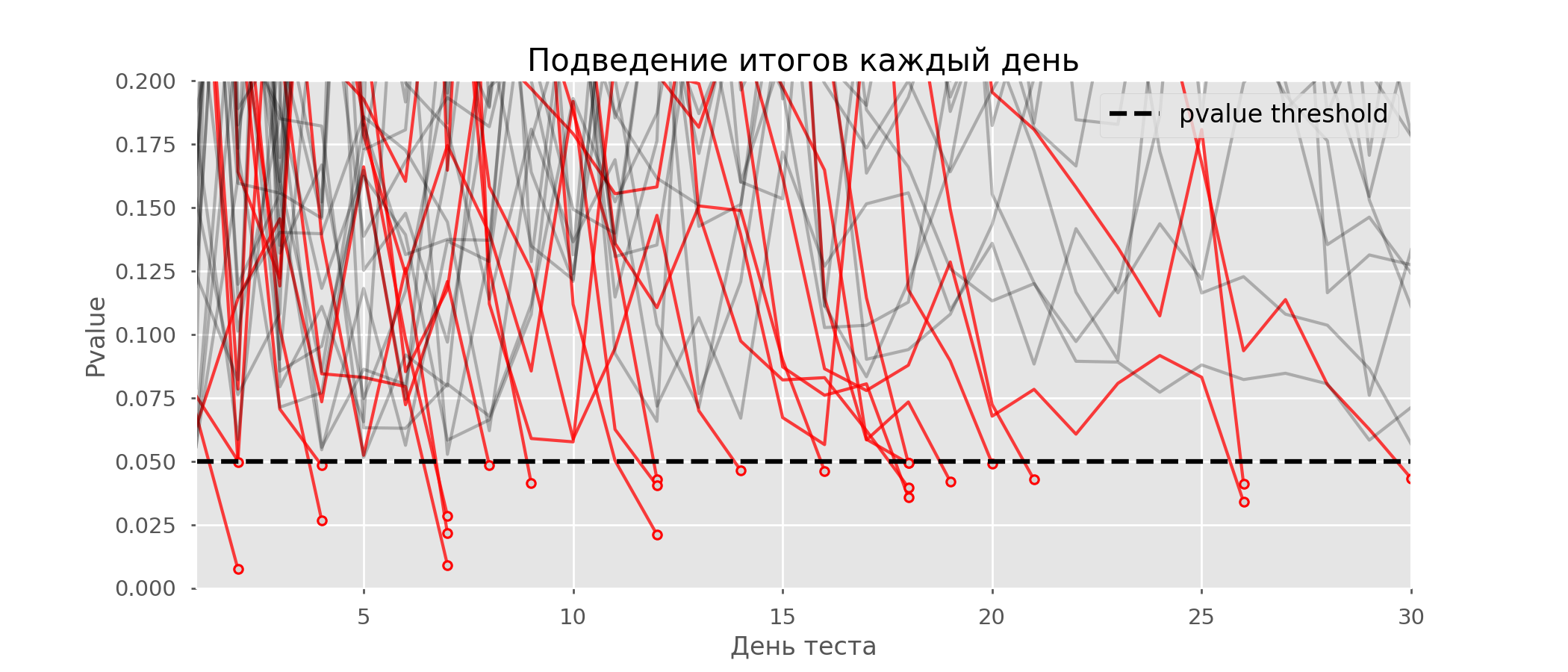There will be a total of 2813 false positive tests out of 10 thousand, or 28%. It is clear that such a scheme is not viable.

Although the problem of peeping is a special case of multiple testing, it’s not worthwhile to apply standard corrections (Bonferroni and others) because they will turn out to be overly conservative. The graph below shows the percentage of false positive results depending on the number of tested groups (red line) and the number of peeps (green line).

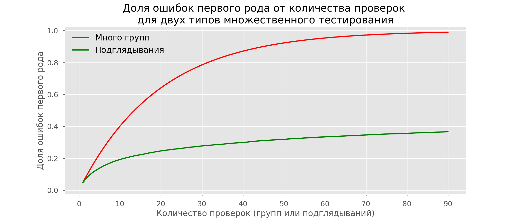Although at infinity and in peeping we come close to 1, the proportion of errors grows much more slowly. This is because the comparisons in this case are no longer independent.

Bayesian Approach and the Peeping Problem

, A/B- . , . .

Early Test Methods

There are test options that allow you to prematurely take the test. I’ll tell you about two of them: with a constant level of significance (Pocock correction) and dependent on the number of peeps (O'Brien-Fleming correction). Strictly speaking, for both corrections you need to know in advance the maximum test period and the number of checks between the start and end of the test. Moreover, checks should occur at approximately equal intervals of time (or at equal amounts of observations).

Pocock

The method is that we summarize the results of the tests every day, but with a reduced (more stringent) level of significance. For example, if we know that we will do no more than 30 checks, then the significance level should be set equal to 0.006 (selected depending on the number of peeps using the Monte Carlo method, i.e. empirically). In our simulation, we get 4% false positive outcomes - apparently, the threshold could be increased.

Despite the apparent naivety, some large companies use this particular method. It is very simple and reliable if you make decisions on sensitive metrics and on a lot of traffic. For example, in Avito, by default , the significance level is set to 0.005 .

O'Brien-Fleming

In this method, the significance level varies depending on the verification number. It is necessary to determine in advance the number of steps (or peeps) in the test and calculate the significance level for each of them. The sooner we try to complete the test, the more stringent the criteria will be applied. Student statistics thresholds

Z_{s t e p}

$Z_{step}$ (including the value in the last step

Z_{l a s t_s t e p}

$Z_{last\_step}$ ) corresponding to the desired significance level depend on the verification number

s t e p_n u m b e r

$step\_number$ (takes values from 1 to the total number of checks

t o t a l_s t e p s

$total\_steps$ inclusive) and are calculated according to the empirically obtained formula:

Z_{l a s t_s t e p} = 2.2471 + \frac{0.3373}{t o t a l_s t e p s} - \frac{0.6331}{\sqrt{t o t a l_s t e p s}} Z_{s t e p} = Z_{l a s t_s t e p} \sqrt{\frac{t o t a l_s t e p s}{s t e p_n u m b e r}}

$Z_{last\_step} = 2.2471 + \frac {0.3373} {total\_steps} − \frac {0.6331} {\sqrt {total\_steps}} \\ Z_{step} = Z_{last\_step} \ {\sqrt { \frac {total\_steps} {step\_number}}}$

Odds code

from sklearn.linear_model import LinearRegression
from sklearn.metrics import explained_variance_score
import matplotlib.pyplot as plt

# datapoints from https://www.aarondefazio.com/tangentially/?p=83
total_steps = [
    2, 3, 4, 5, 6, 8, 10, 15, 20, 25, 30, 50, 60
]
last_z = [
    1.969, 1.993, 2.014, 2.031, 2.045, 2.066, 2.081, 
    2.107, 2.123, 2.134, 2.143, 2.164, 2.17
]
features = [
    [1/t, 1/t**0.5] for t in total_steps
]
lr = LinearRegression()
lr.fit(features, last_z)
print(lr.coef_)  # [ 0.33729346, -0.63307934]
print(lr.intercept_)  # 2.247105015502784
print(explained_variance_score(lr.predict(features), last_z))  # 0.999894

total_steps_extended = np.arange(2, 80)
features_extended = [ [1/t, 1/t**0.5] for t in total_steps_extended ]
plt.plot(total_steps_extended, lr.predict(features_extended))
plt.scatter(total_steps, last_z, s=30, color='black')
plt.show()

The relevant significance levels are calculated through the percentile

p e r c

$perc$ standard distribution corresponding to the value of student statistics

Z

$Z$ :

perc = scipy.stats.norm.cdf(Z)
pval_thresholds = (1 − perc) * 2

On the same simulations, it looks like this:

False-positive results were 501 out of 10 thousand, or the expected 5%. Please note that the significance level does not reach a value of 5% even at the end, since these 5% should be "smeared" over all checks. At the company, we use this very correction if we run a test with the possibility of an early stop. You can read about the same and other amendments here .

Optimizely Method

Optimizely , , . , . , . O'Brien-Fleming’a .

A / B Test Calculator

The specifics of our product is such that the distribution of any metric varies greatly depending on the audience of the test (for example, class number) and the time of year. Therefore, it will not be possible to accept the rules for the end date of the test in the spirit of “the test will end when 1 million users are typed in each group” or “the test will end when the number of solved tasks reaches 100 million”. That is, it will work, but in practice, for this, it will be necessary to take into account too many factors:

what classes get into the test;
the test is distributed to teachers or students;
academic year time;
test for all users or only for new ones.

However, in our A / B testing schemes, you always need to fix the end date in advance. To predict the duration of the test, we developed an internal application - A / B test calculator. Based on the activity of users from the selected segment over the past year, the application calculates the period for which the test must be run in order to significantly fix the uplift in X% by the selected metric. The correction for multiple tests is also automatically taken into account and threshold significance levels are calculated for an early test stop.

All metrics are calculated at the level of test objects. If the metric is the number of problems solved, then in the test at the teacher level this will be the sum of the problems solved by his students. Since we use the student criterion, we can pre-calculate the aggregates needed by the calculator for all possible slices. For each day from the start of the test, you need to know the number of people in the test

u s e r s_c n t

$users\_cnt$ , the average value of the metric

m e t r i c_m e a n

$metric\_mean$ and its variance

m e t r i c_s t d

$metric\_std$ . Fixing the shares of the control group

c o n t r o l_g r o u p_s h a r e

$control\_group\_share$ experimental group

e x p_g r o u p_s h a r e

$exp\_group\_share$ and expected gain from the test

u p l i f t_e x p e c t e d

$uplift\_expected$ in percent, you can calculate the expected values of student statistics

t t e s t_s t a t_v a l u e

$ttest\_stat\_value$ and the corresponding p-value for each day of the test:

t t e s t_s t a t_p r e c u r s o r = \frac{m e t r i c_m e a n \sqrt{u s e r s_c n t}}{m e t r i c_s t d} t t e s t_s t a t_v a l u e = \frac{t t e s t_s t a t_p r e c u r s o r}{\sqrt{\frac{1}{c o n t r o l_g r o u p_s h a r e} + \frac{1}{e x p_g r o u p_s h a r e}}} * u p l i f t_e x p e c t e d / 100

$ttest\_stat\_precursor = \frac{metric\_mean\ \sqrt {users\_cnt}}{metric\_std} \\ ttest\_stat\_value = \frac {ttest\_stat\_precursor} {\sqrt{ \frac{1} {control\_group\_share} + \frac {1} {exp\_group\_share}}} * uplift\_expected / 100$

Next, it's easy to get p-values for each day:

pvalue = (1 − scipy.stats.norm.cdf(ttest_stat_value)) * 2

Knowing the p-value and significance level, taking into account all the corrections for each day of the test, for any duration of the test, you can calculate the minimum uplift that can be detected (in the English literature - MDE, minimal detectable effect). After that, it is easy to solve the inverse problem - to determine the number of days required to identify the expected uplift.

Conclusion

In conclusion, I want to recall the main messages of the article:

If you compare the average values of the metric in groups, most likely, the Student criterion will suit you. The exception is extremely small sample sizes (dozens of observations) or abnormal metric distributions (in practice, I have not seen such).
If there are several groups in the test, use corrections for multiple hypothesis testing. The simplest Bonferroni correction will do.
.
. .
. , , , , O'Brien-Fleming.
A/B-, A/A-.

Despite all of the above, business and common sense should not suffer for the sake of mathematical rigor. Sometimes it is possible to roll out functional for all that did not show a significant increase in the test, some changes inevitably occur without testing at all. But if you conduct hundreds of tests a year, their accurate analysis is especially important. Otherwise, there is a risk that the number of false positive tests will be comparable to really useful ones.

What we pay attention to when calculating the statistical significance of the A / B test