Fuzzy logic and state machines against the PID controller. Beating the babies continues

We continue to study fuzzy logic according to the book by V. Gostev, “Fuzzy Controllers in Automatic Control Systems”. After we enjoyed the beautiful views of the response surfaces , we proceed directly to solving the next problem from V. Gostev’s book “Fuzzy Regulators in Automatic Control Systems”.

This text is a continuation of previous publications:

1. A simple controller based on fuzzy logic. Creation and customization.
2. Fuzzy logic in beautiful pictures. Response surfaces for different membership functions.
3. Creating a controller based on fuzzy logic with multi-channel settings.
4. Simple fuzzy logic is molded “from what was” for a gas turbine engine.
5. Fuzzy logic against PID. We cross the hedgehog and the snake. Aircraft engine and NPP control algorithms.

For those who are unfamiliar with fuzzy logic, I recommend that you first read the first text, after that, everything that is described below will be simple and clear.

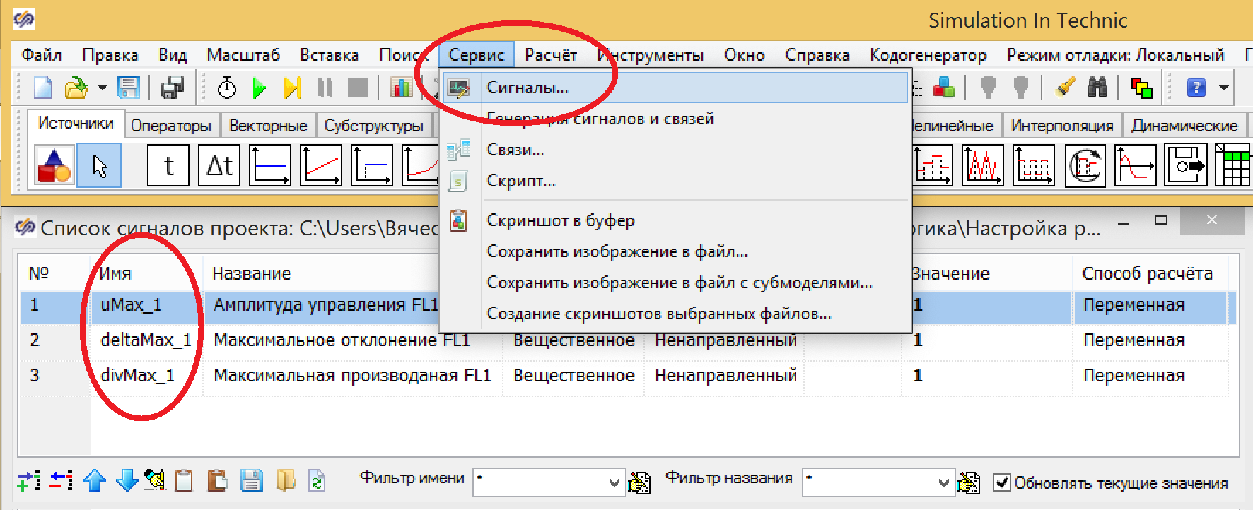
, - . , . , Fuzzy. , , . , , , , .

, , , .

– -, (). , , « . »

, , , 1 ( ).

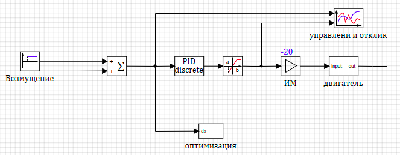
1. .

.
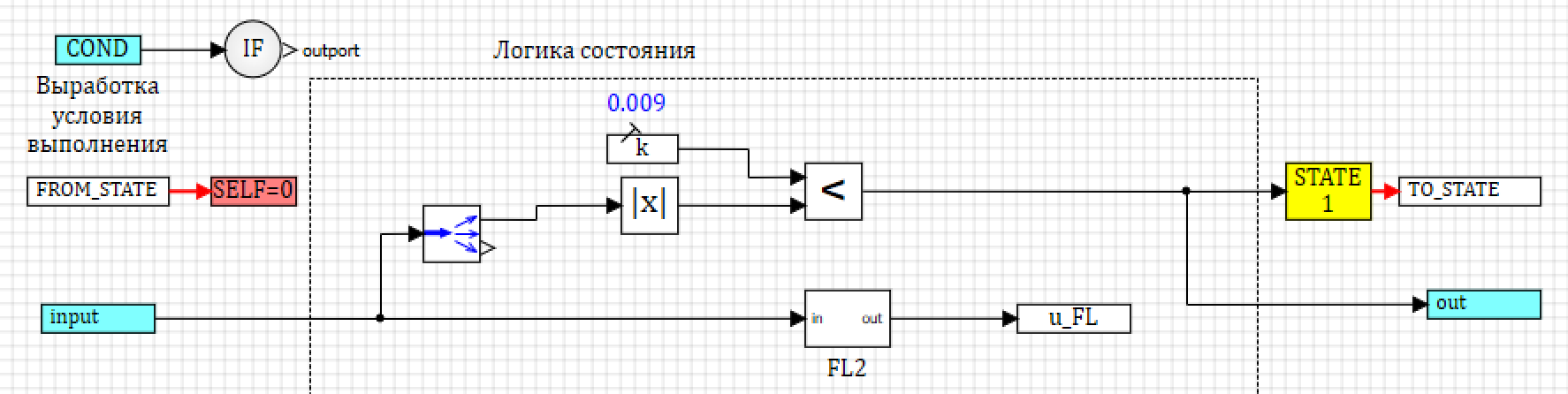
. 1 . , . – , .

: – , – . , 0.009 .

, -.

, 2. – 20, (- «as is» .. ).

2. .

- 0.001 0.001.

- 1,1,1 . 3.

, , 1 1000, 0,001. , . , -1 1 , 0 7 .

What can you say by looking at this chart? Never mind. And all because our model is already presented as a transfer function in deviations, and we can’t say whether it is fast or not. We can’t say anything about the engine. As I have already shown in the article “Technology for obtaining dynamic equations of TAU. And why is System Identification is sucks, and “honest physics” rules : the transformation of a parametric physical system to a kind of transfer function ruins the whole engineering “understandability” of the model.
For example, is the impact on a model with a value of 1000 obtained after PID possible in life? Unknown If this is a fuel supply, then it is obvious that the supply system will not be able to cram 1000 times more fuel than in idle mode.

, 10, -10. . , . :

4. .

, , ( 5). 1000, , 10.

5. .

.
C . 0

6. .

7.

7. ..

. :
— – , 0.009.
— .

«-3» . , , , — .

« » .

, , . , .

, « » , , .. .

, , . , .
, . , , , .

8.

8. .

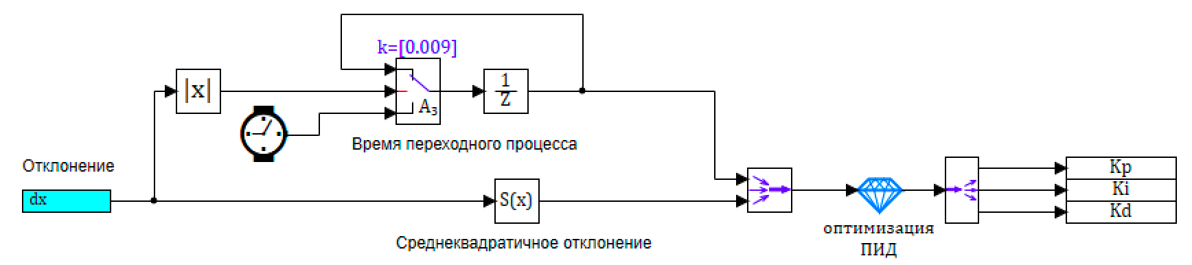
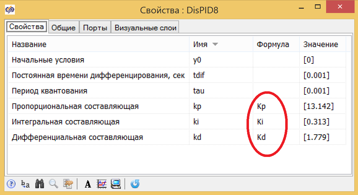
. , , . p, Ki, Kd (. . 7 . 8). -. (. 10.)

9. .

10. -.

:
Kp = 13.142
Ki = 0.313
Kd = 1.779
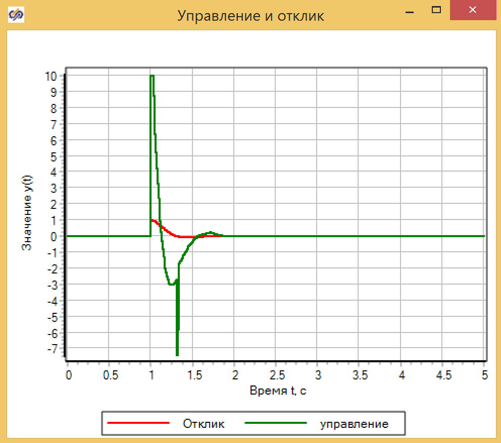
0.72 . 11.

11. -.

, .

1 , . .

The incoming deviation signals and the rate of variation of the deviation, passing through the phasing units, are decomposed into three terms each. Using the Gauss membership functions.

Deviation - more , norm , less .
The rate of change is growing , not changing , falling .

The regulator will give an effect when a deviation appears, and also when the rate of change of the regulator indicates that the deviation will increase (even if at the moment it is normal). Base rules for the regulator:

1. ( (0) ), .
2. , 0.
3. ( (0) ), .

, , 12.

12. Fuzzy Logic.

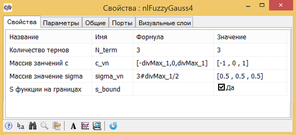
. , 0, . :

• uMax_1 – ;
• deltaMax_1 – ;
• divMax_1 – .

– . 13.

13. .

(–uMax_1… uMax_1) [–uMax_1 ,0, uMax_1], , 2. (. , ).

, :

14. .

.
, :

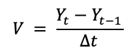where:
Y _t is the current value;
Y _t-1 is the value in the previous step;
Δt = 0.001 - time step is the same as when sampling a discrete PID controller.

The circuit is shown in Figure 15. The division by Δt is taken into account in the comparison block, where the coefficients for each input can be set.

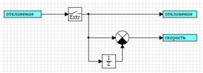
Figure 16. Scheme for calculating the rate of change.

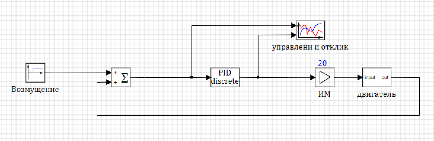
Since the entire circuit is ready for us, it remains to replace the PID controller with the FL controller (see Figure 17) and see what happens.

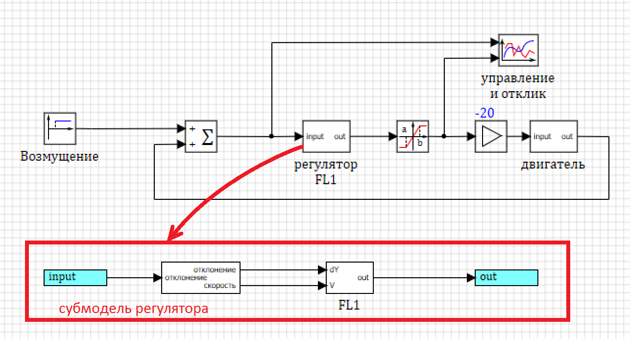
Figure 17. Diagram of a model with one fuzzy controller.

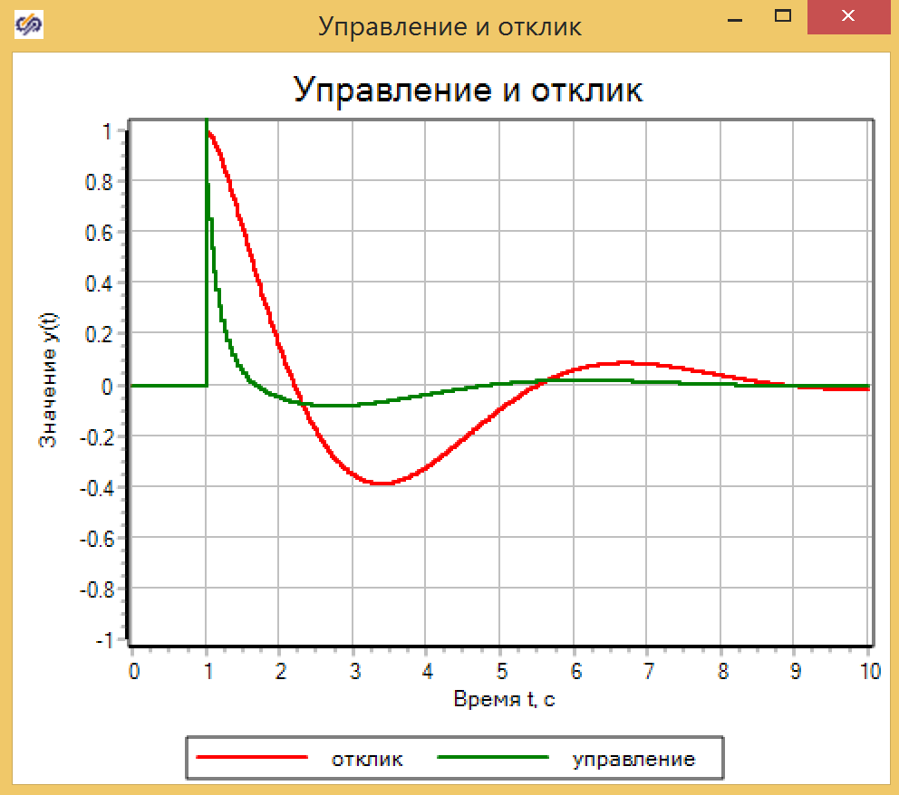
And again, to my considerable surprise, the fuzzy controller did better than the PID in the initial single settings. Some kind of continuous advertising of fuzzy logic is obtained.

Moreover, if in previous cases it could be attributed to the fact that the second derivative is used in the fuzzy controller, then in this case this fuzzy controller uses the same derivative, and the PID also uses the integral component.

So that advocates of gender diversity do not accuse me of oppressing traditional PID regulators, the coefficient of the integral component is nullified and a PD regulator is obtained. The result has improved significantly, but FL is still better.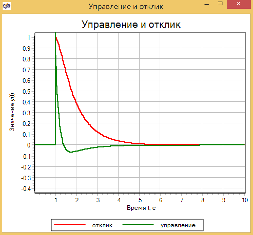

Figure 19. PD controller with single settings.

, 0.009. :
– 11.25 .
— 5.25 .
FL – 4.74 .

FL

, - (. 6). :
— uMax_1 – ;
— deltaMax_1 – ;
— divMax_1 – .

1. .

, .

20. .

, , .

. .

21. .

0.24
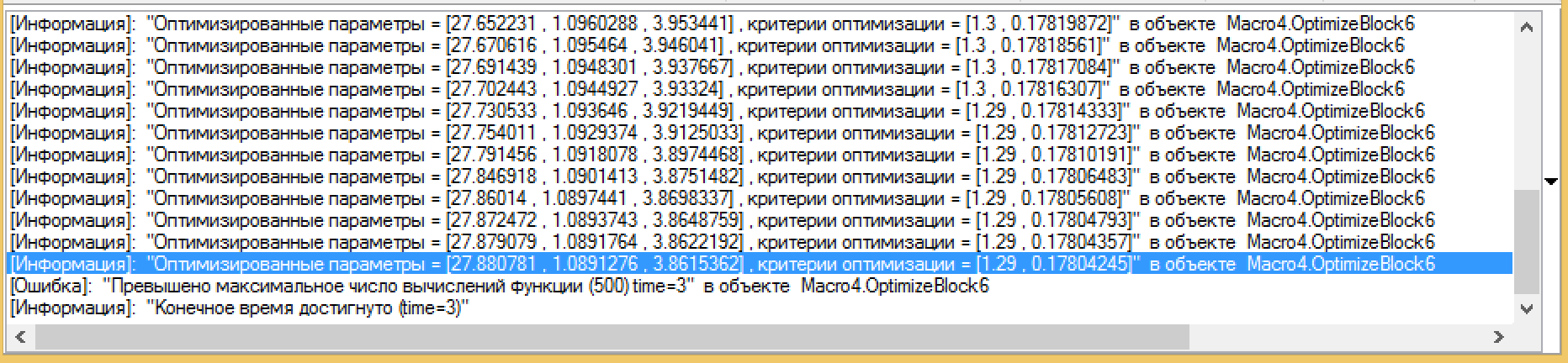
[]: « = [31.10359, 1.0219553, 2.165446], = [1.24, 0.09879439]» Macro4.OptimizeBlock6

0.23 .
[]: « = [34.954824, 1.0114662, 0.058949452], = [1.23, 0.098544697]» Macro4.OptimizeBlock6

FL 22. , .

, .

, . . , , , .

, , , .

. – SimInTech, - , .

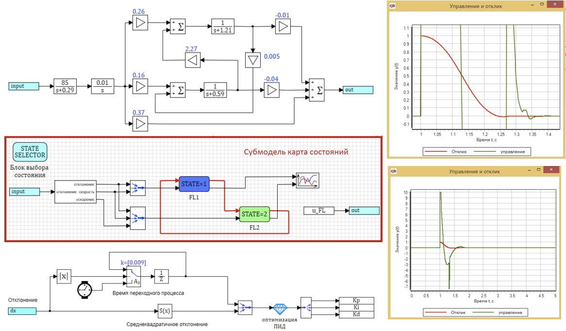
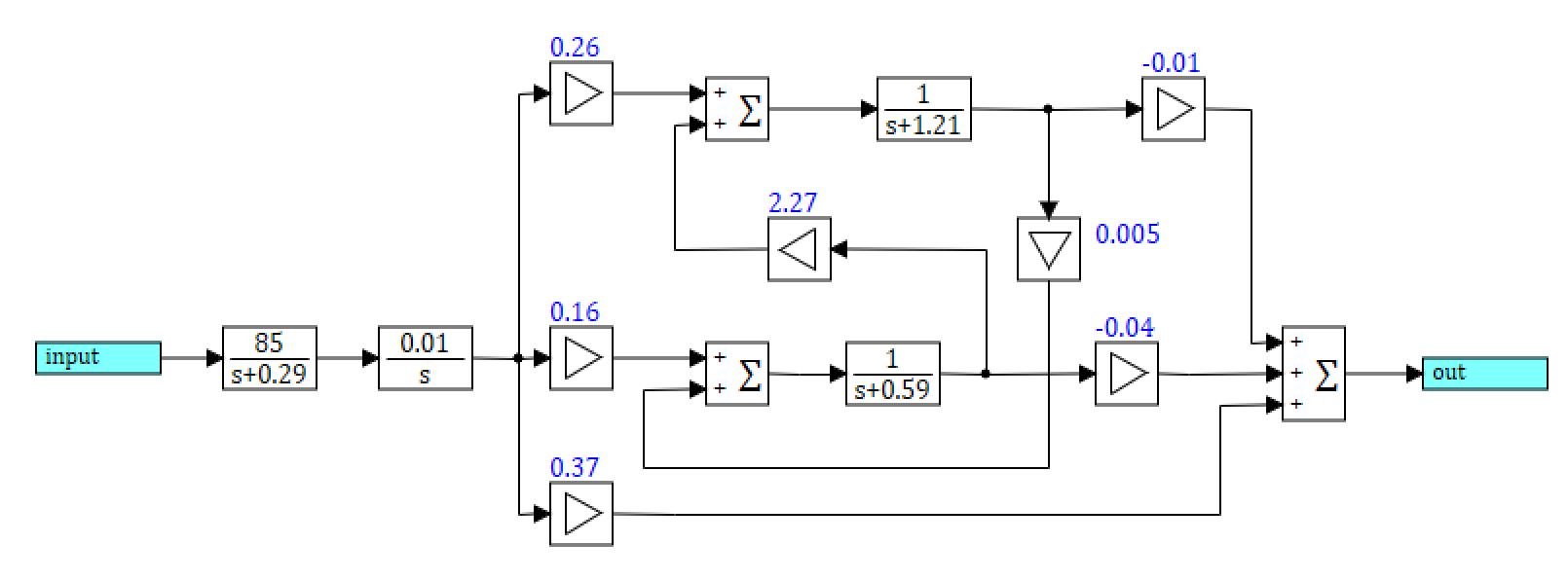
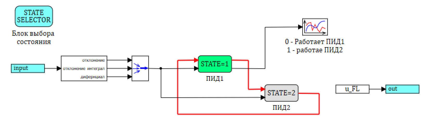
. . – FL1, — FL2. , 23:

23. .

, , – , .

, .

, , , , . .

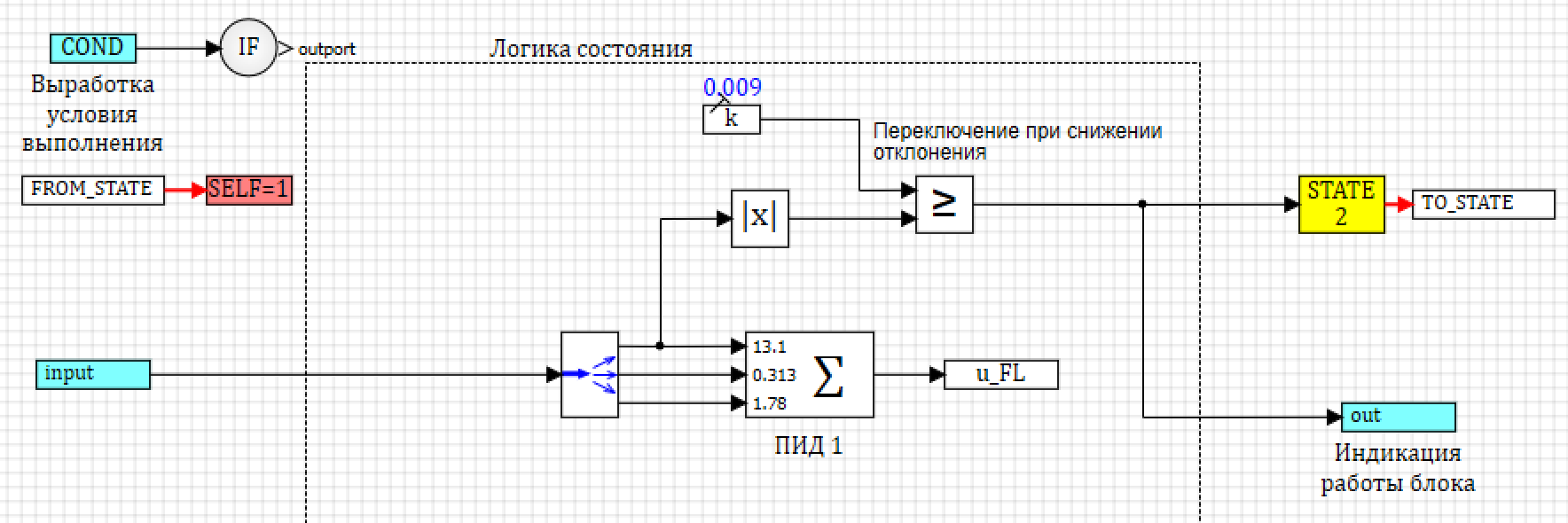
, , , «1 », , 0.001 ( ). . — .

, , , (), . , , 1000 , 1 000 000 . . . 24.

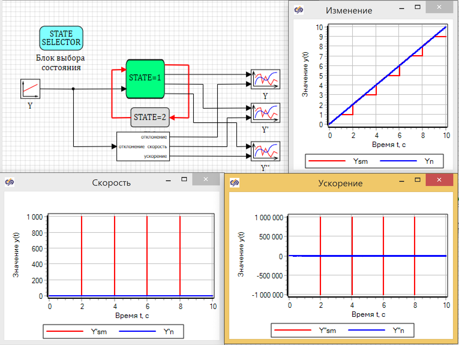
24. .

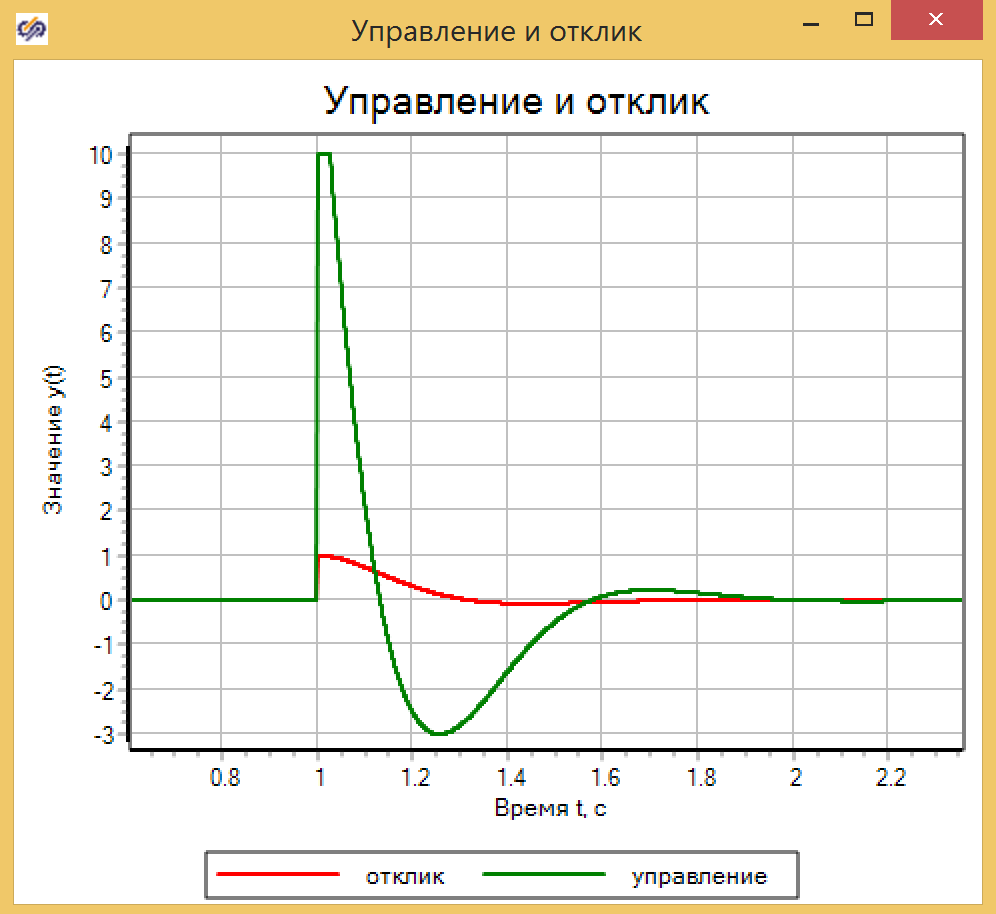
: , 0.009. , , .

FL1, . , u_FL. , , .

25. 1.

– , 1 , 0.009.

26. 2.

( .. ). 24.

, , u_FL FL1, FL2 .

. , . , . , , .

– , , .
– , , .
— , , .

, :

1) if the deviation is greater and the rate of change increases and the acceleration of change accelerates , then the effect is reduced .
2) if the deviation is normal and the rate of change is constant and the acceleration of change does not change , then the effect does not change .
3) if the deviation is less and the rate of change decreases and the acceleration of change slows down , then impact increase .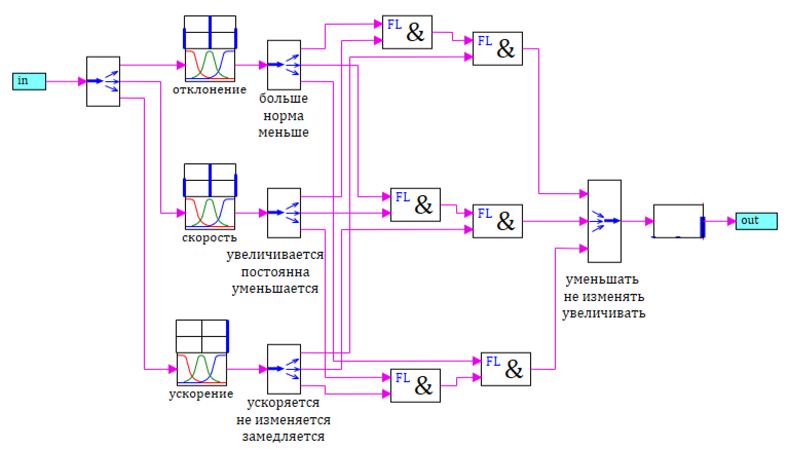

27. FL2.

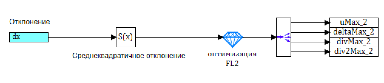
N , , 0, .
:
— uMax_2 – ;
— deltaMax_2 – ;
— divMax_2 – ;
— div2Max_2 – .

1 (. . 28)
1 , - , , 1 (. . 18 — 19) – , . . (. . 28)

28. .

: , . 29, – 30.

29. .

30. .

, . , . , .

, . .
:
sign, -1,0,1 , « », 1 . , , .
, .

, , 1.2 , .

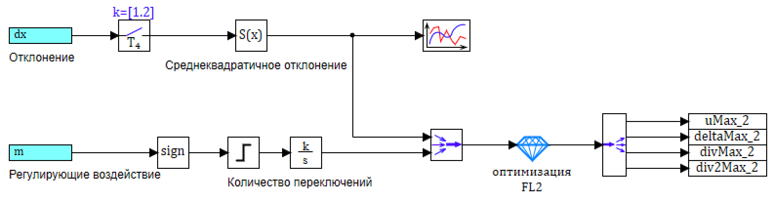
31. ee.

:

[]: « = [16.564415, 0.0027674129, 0.19085771, 50], = [0.0047956855, 11]» Macro5.OptimizeBlock6

, :
— uMax_2 – = 16.564;
— deltaMax_2 – = 0.00277;
— divMax_2 – = 0.191;
— div2Max_2 – = 50.
32.

, , , . 1, 2 , .

33. , , .

33. 1 2.

, , , . . 34.

34. -.

2, , . - :

35. -.

:

, , .

...