 The last couple of years in my free time I have been doing triathlon. This sport is very popular in many countries of the world, especially in the USA, Australia and Europe. Currently gaining rapid popularity in Russia and the CIS countries. It is about involving amateurs, not professionals. Unlike just swimming in the pool, cycling and jogging in the morning, a triathlon involves participating in competitions and systematic preparation for them, even without being a professional. Surely among your friends there is already at least one “iron man” or someone who plans to become one. Massiveness, a variety of distances and conditions, three sports in one - all this has the potential for the formation of a large amount of data. Each year, several hundred triathlon competitions take place in the world, in which several hundred thousand people participate.Competitions are held by several organizers. Each of them, naturally, publishes the results in its own right. But for athletes from Russia and some CIS countries, the teamtristats.ru collects all the results in one place - on its website of the same name. This makes it very convenient to search for results, both yours and your friends and rivals, or even your idols. But for me it also gave the opportunity to analyze a large number of results programmatically. Results published on trilife: read .This was my first project of this kind, because only recently I started doing data analysis in principle, as well as using python. Therefore, I want to tell you about the technical implementation of this work, especially since in the process, various nuances surfaced, sometimes requiring a special approach. It will be about scraping, parsing, casting types and formats, restoring incomplete data, creating a representative sample, visualization, vectorization, and even parallel computing.The volume turned out to be large, so I broke everything into five parts so that I could dose out the information and remember where to start after the break.Before moving on, it is better to first read my article with the results of the study, because here essentially described the kitchen for its creation. It takes 10-15 minutes.Have you read? Then let's go!
Part 1. Scraping and parsing
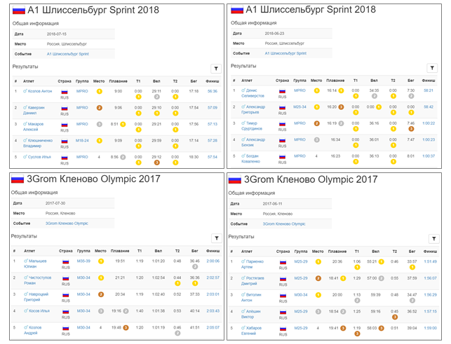
Given: Website tristats.ru . There are two types of tables on it that interest us. This is actually a summary table of all races and a protocol of the results of each of them.
 The number one task was to obtain this data programmatically and save it for further processing. It so happened that at that time I was new to web technologies and therefore did not immediately know how to do this. I started accordingly with what I knew - look at the page code. This can be done using the right mouse button or the F12 key .
 The menu in Chrome contains two options: View page code and View code . Not the most obvious division. Naturally, they give different results. The one that view the code, it’s just the same as F12 - the directly textual html- representation of what is displayed in the browser is element-wise.
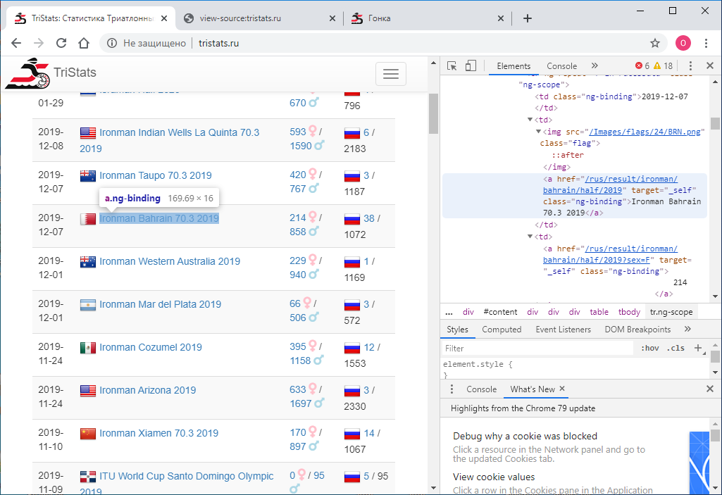 In turn, viewing the page code gives the source code of the page. Also html , but there is no data there, only the names of the JS scripts that unload them. Okay.
 Now we need to understand how to use python to save the code of each page as a separate text file. I try this:
import requests

r = requests.get(url='http://tristats.ru/')
print(r.content)
And I get ... the source code. But I need the result of its execution. After studying, searching and asking around, I realized that I needed a tool to automate browser actions, for example, selenium . I put it. And also ChromeDriver for work with Google Chrome . Then I used it as follows:from selenium import webdriver
from selenium.webdriver.chrome.service import Service
service = Service(r'C:\ChromeDriver\chromedriver.exe')
service.start()
driver = webdriver.Remote(service.service_url)
driver.get('http://www.tristats.ru/')
print(driver.page_source)
driver.quit()
This code launches a browser window and opens a page in it at the specified url. As a result, we get html code already with the desired data. But there is one snag. The result is only 100 entries, and the total number of races is almost 2000. How so? The fact is that initially only the first 100 entries are displayed in the browser, and only if you scroll to the very bottom of the page, the next 100 are loaded, and so on. Therefore, it is necessary to implement scrolling programmatically. To do this, use the command:driver.execute_script("window.scrollTo(0, document.body.scrollHeight);")
And with each scrolling, we will check whether the code of the loaded page has changed or not. If it hasn’t changed, we’ll check several times for reliability, for example 10, then the whole page is loaded and you can stop. Between the scrolls we set the timeout to one second so that the page has time to load. (Even if she doesn’t have time, we have a reserve - another nine seconds).And the full code will look like this:from selenium import webdriver
from selenium.webdriver.chrome.service import Service
import time
service = Service(r'C:\ChromeDriver\chromedriver.exe')
service.start()
driver = webdriver.Remote(service.service_url)
driver.get('http://www.tristats.ru/')
prev_html = ''
scroll_attempt = 0
while scroll_attempt < 10:
driver.execute_script("window.scrollTo(0, document.body.scrollHeight);")
time.sleep(1)
if prev_html == driver.page_source:
scroll_attempt += 1
else:
prev_html = driver.page_source
scroll_attempt = 0
with open(r'D:\tri\summary.txt', 'w') as f:
f.write(prev_html)
driver.quit()
So, we have an html file with a summary table of all races. Need to parse it. To do this, use the lxml library .from lxml import html
First we find all the rows of the table. To determine the sign of a string, just look at the html file in a text editor. It can be, for example, “tr ng-repeat = 'r in racesData' class = 'ng-scope'” or some fragment that can no longer be found in any tags.
with open(r'D:\tri\summary.txt', 'r') as f:
    sum_html = f.read()

tree = html.fromstring(sum_html)
rows = tree.findall(".//*[@ng-repeat='r in racesData']")
then we start pandas dataframe and each element of each row of the table is written to this dataframe.import pandas as pd
rs = pd.DataFrame(columns=['date','name','link','males','females','rus','total'], index=range(len(rows)))
In order to figure out where each specific element is hidden, you just need to look at the html code of one of the elements of our rows in the same text editor.<tr ng-repeat="r in racesData" class="ng-scope">
<td class="ng-binding">2015-04-26</td>
<td>
<img src="/Images/flags/24/USA.png" class="flag">
<a href="/rus/result/ironman/texas/half/2015" target="_self" class="ng-binding">Ironman Texas 70.3 2015</a>
</td>
<td>
<a href="/rus/result/ironman/texas/half/2015?sex=F" target="_self" class="ng-binding">605</a>
<i class="fas fa-venus fa-lg" style="color:Pink"></i>
/
<a href="/rus/result/ironman/texas/half/2015?sex=M" target="_self" class="ng-binding">1539</a>
<i class="fas fa-mars fa-lg" style="color:LightBlue"></i>
</td>
<td class="ng-binding">
<img src="/Images/flags/24/rus.png" class="flag">
<a ng-if="r.CountryCount > 0" href="/rus/result/ironman/texas/half/2015?country=rus" target="_self" class="ng-binding ng-scope">2</a>
/ 2144
</td>
</tr>
The easiest way to hardcode navigation for children here is that there are not many of them.for i in range(len(rows)):
rs.loc[i,'date'] = rows[i].getchildren()[0].text.strip()
rs.loc[i,'name'] = rows[i].getchildren()[1].getchildren()[1].text.strip()
rs.loc[i,'link'] = rows[i].getchildren()[1].getchildren()[1].attrib['href'].strip()
rs.loc[i,'males'] = rows[i].getchildren()[2].getchildren()[2].text.strip()
rs.loc[i,'females'] = rows[i].getchildren()[2].getchildren()[0].text.strip()
rs.loc[i,'rus'] = rows[i].getchildren()[3].getchildren()[3].text.strip()
rs.loc[i,'total'] = rows[i].getchildren()[3].text_content().split('/')[1].strip()
Here is the result: Save this data frame to a file. I use pickle , but it could be csv , or something else.import pickle as pkl
with open(r'D:\tri\summary.pkl', 'wb') as f:
pkl.dump(df,f)
At this stage, all data is of a string type. We will convert later. The most important thing we need now is links. We will use them for scraping protocols of all races. We make it in the image and likeness of how it was done for the pivot table. In the cycle for all races for each, we will open the page by reference, scroll and get the page code. In the summary table we have information on the total number of participants in the race - total, we will use it in order to understand until what point you need to continue to scroll. To do this, we will directly in the process of scraping each page determine the number of records in the table and compare it with the expected value of total. As soon as it is equal, then we scrolled to the end and you can proceed to the next race. We also set a timeout of 60 seconds. Ate during this time, we do not get to total , go to the next race. The page code will be saved to a file. We will save the files of all races in one folder, and name them by the name of the races, that is, by the value in the event column in the summary table. To avoid a conflict of names, it is necessary that all races have different names in the pivot table. Check this:df[df.duplicated(subset = 'event', keep=False)]
service.start()
driver = webdriver.Remote(service.service_url)
timeout = 60

for index, row in df.iterrows():
    try:
        driver.get('http://www.tristats.ru' + row['link'])
        start = time.time()

        while True:
            driver.execute_script("window.scrollTo(0, document.body.scrollHeight);")
            time.sleep(1)
            race_html = driver.page_source
            tree = html.fromstring(race_html)
            race_rows = tree.findall(".//*[@ng-repeat='r in resultsData']")

            if len(race_rows) == int(row['total']):
                break
            if time.time() - start > timeout:
                print('timeout')
                break

        with open(os.path.join(r'D:\tri\races', row['event'] +  '.txt'), 'w') as f:
            f.write(race_html)

    except:
        traceback.print_exc()

    time.sleep(1)

driver.quit()
This is a long process. But when everything is set up and this heavy mechanism starts spinning, adding data files one after another, a feeling of pleasant excitement comes. Only about three protocols are loaded per minute, very slowly. Left to spin for the night. It took about 10 hours. By morning, most of the protocols were uploaded. As it usually happens when working with a network, a few fail. Quickly resumed them with a second attempt.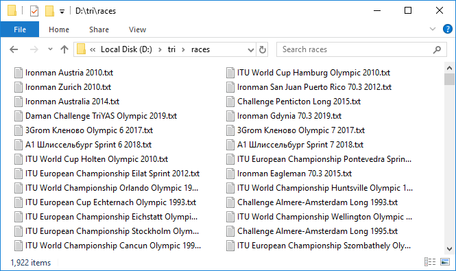 So, we have 1,922 files with a total capacity of almost 3 GB. Cool! But handling almost 300 races ended in a timeout. What is the matter? Selectively check, it turns out that indeed the total value from the pivot table and the number of entries in the race protocol that we checked may not coincide. This is sad because it is not clear what is the reason for this discrepancy. Either this is due to the fact that not everyone will finish, or some kind of bug in the database. In general, the first signal of data imperfection. In any case, we check those in which the number of entries is 100 or 0, these are the most suspicious candidates. There were eight of them. Download them again under close control. By the way, in two of them there are actually 100 entries.Well, we have all the data. We pass to parsing. Again, in a cycle we will run through each race, read the file and save the contents in a pandas DataFrame . We will combine these data frames into a dict , in which the names of the races are the keys - that is, the event values from the pivot table or the names of the files with the html code of the race pages, they coincide.
rd = {}
for e in rs['event']:
place = []
... sex = [], name=..., country, group, place_in_group, swim, t1, bike, t2, run
result = []
with open(os.path.join(r'D:\tri\races', e + '.txt'), 'r')
race_html = f.read()
tree = html.fromstring(race_html)
rows = tree.findall(".//*[@ng-repeat='r in resultsData']")
for j in range(len(rows)):
row = rows[j]
parts = row.text_content().split('\n')
parts = [r.strip() for r in parts if r.strip() != '']
place.append(parts[0])
if len([a for a in row.findall('.//i')]) > 0:
sex.append([a for a in row.findall('.//i')][0].attrib['ng-if'][10:-1])
else:
sex.append('')
name.append(parts[1])
if len(parts) > 10:
country.append(parts[2].strip())
k=0
else:
country.append('')
k=1
group.append(parts[3-k])
... place_in_group.append(...), swim.append ..., t1, bike, t2, run
result.append(parts[10-k])
race = pd.DataFrame()
race['place'] = place
... race['sex'] = sex, race['name'] = ..., 'country', 'group', 'place_in_group', 'swim', ' t1', 'bike', 't2', 'run'
race['result'] = result
rd[e] = race
with open(r'D:\tri\details.pkl', 'wb') as f:
pkl.dump(rd,f)
for index, row in rs.iterrows():
    e = row['event']
    with open(os.path.join(r'D:\tri\races', e + '.txt'), 'r') as f:
        race_html = f.read()

    tree = html.fromstring(race_html)
    header_elem = [tb for tb in tree.findall('.//tbody') if tb.getchildren()[0].getchildren()[0].text == ''][0]
    location = header_elem.getchildren()[1].getchildren()[1].text.strip()
    rs.loc[index, 'loc'] = location
with open(r'D:\tri\summary1.pkl', 'wb') as f:
    pkl.dump(df,f)
Part 2. Type casting and formatting
So, we downloaded all the data and put it in the data frames. However, all values are of type str . This applies to the date, and to the results, and to the location, and to all other parameters. All parameters must be converted to the appropriate types.Let's start with the pivot table.date and time
event , loc and link will be left as is. date convert to pandas datetime as follows:rs['date'] = pd.to_datetime(rs['date'])
The rest are cast to an integer type:cols = ['males', 'females', 'rus', 'total']
rs[cols] = rs[cols].astype(int)
Everything went smoothly, no errors arose. So everything is OK - save:with open(r'D:\tri\summary2.pkl', 'wb') as f:
pkl.dump(rs, f)
Now racing dataframes. Since all races are more convenient and faster to process at once, and not one at a time, we will collect them into one large ar data frame (short for all records ) using the concat method .ar = pd.concat(rd)
ar contains 1,416,365 entries.Now convert place and place in group to an integer value.ar[['place', 'place in group']] = ar[['place', 'place in group']].astype(int))
Next, we process the columns with temporary values. We will cast them in the type Timedelta from pandas . But for the conversion to succeed, you need to properly prepare the data. You can see that some values that are less than an hour go without specifying the very tip. Need to add it.for col in ['swim', 't1', 'bike', 't2', 'run', 'result']:
strlen = ar[col].str.len()
ar.loc[strlen==5, col] = '0:' + ar.loc[strlen==5, col]
ar.loc[strlen==4, col] = '0:0' + ar.loc[strlen==4, col]
Now times, still remaining strings, look like this: Convert to Timedelta :for col in ['swim', 't1', 'bike', 't2', 'run', 'result']:
ar[col] = pd.to_timedelta(ar[col])
Floor
Move on. Check that in the sex column there are only the values of M and F :ar['sex'].unique()
Out: ['M', 'F', '']
In fact, there is still an empty string, that is, the gender is not specified. Let's see how many such cases:len(ar[ar['sex'] == ''])
Out: 2538
Not so much is good. In the future, we will try to further reduce this value. In the meantime, leave the sex column as is in the form of lines. We will save the result before moving on to more serious and risky transformations. In order to maintain continuity between files, we transform the combined data frame ar back into the dictionary of data frames rd :for event in ar.index.get_level_values(0).unique():
rd[event] = ar.loc[event]
with open(r'D:\tri\details1.pkl', 'wb') as f:
pkl.dump(rd,f)
By the way, due to the conversion of the types of some columns, file sizes decreased from 367 KB to 295 KB for the pivot table and from 251 MB to 168 MB for racing protocols.Country code
Now let's see the country.ar['country'].unique()
Out: ['CRO', 'CZE', 'SLO', 'SRB', 'BUL', 'SVK', 'SWE', 'BIH', 'POL', 'MK', 'ROU', 'GRE', 'FRA', 'HUN', 'NOR', 'AUT', 'MNE', 'GBR', 'RUS', 'UAE', 'USA', 'GER', 'URU', 'CRC', 'ITA', 'DEN', 'TUR', 'SUI', 'MEX', 'BLR', 'EST', 'NED', 'AUS', 'BGI', 'BEL', 'ESP', 'POR', 'UKR', 'CAN', 'IRL', 'JPN', 'HKG', 'JEY', 'SGP', 'BRA', 'QAT', 'LUX', 'RSA', 'NZL', 'LAT', 'PHI', 'KSA', 'SEY', 'MAS', 'OMA', 'ARG', 'ECU', 'THA', 'JOR', 'BRN', 'CIV', 'FIN', 'IRN', 'BER', 'LBA', 'KUW', 'LTU', 'SRI', 'HON', 'INA', 'LBN', 'PAN', 'EGY', 'MLT', 'WAL', 'ISL', 'CYP', 'DOM', 'IND', 'VIE', 'MRI', 'AZE', 'MLD', 'LIE', 'VEN', 'ALG', 'SYR', 'MAR', 'KZK', 'PER', 'COL', 'IRQ', 'PAK', 'CZK', 'KAZ', 'CHN', 'NEP', 'ISR', 'MKD', 'FRO', 'BAN', 'ARU', 'CPV', 'ALB', 'BIZ', 'TPE', 'KGZ', 'BNN', 'CUB', 'SNG', 'VTN', 'THI', 'PRG', 'KOR', 'RE', 'TW', 'VN', 'MOL', 'FRE', 'AND', 'MDV', 'GUA', 'MON', 'ARM', 'F.I.TRI.', 'BAHREIN', 'SUECIA', 'REPUBLICA CHECA', 'BRASIL', 'CHI', 'MDA', 'TUN', 'NDL', 'Danish(Dane)', 'Welsh', 'Austrian', 'Unknown', 'AFG', 'Argentinean', 'Pitcairn', 'South African', 'Greenland', 'ESTADOS UNIDOS', 'LUXEMBURGO', 'SUDAFRICA', 'NUEVA ZELANDA', 'RUMANIA', 'PM', 'BAH', 'LTV', 'ESA', 'LAB', 'GIB', 'GUT', 'SAR', 'ita', 'aut', 'ger', 'esp', 'gbr', 'hun', 'den', 'usa', 'sui', 'slo', 'cze', 'svk', 'fra', 'fin', 'isr', 'irn', 'irl', 'bel', 'ned', 'sco', 'pol', 'SMR', 'mex', 'STEEL T BG', 'KINO MANA', 'IVB', 'TCH', 'SCO', 'KEN', 'BAS', 'ZIM', 'Joe', 'PUR', 'SWZ', 'Mark', 'WLS', 'MYA', 'BOT', 'REU', 'NAM', 'NCL', 'BOL', 'GGY', 'ISV', 'TWN', 'GUM', 'FIJ', 'COK', 'NGR', 'IRI', 'GAB', 'ANT', 'GEO', 'COG', 'sue', 'SUD', 'BAR', 'CAY', 'BO', 'VE', 'AX', 'MD', 'PAR', 'UM', 'SEN', 'NIG', 'RWA', 'YEM', 'PLE', 'GHA', 'ITU', 'UZB', 'MGL', 'MAC', 'DMA', 'TAH', 'TTO', 'AHO', 'JAM', 'SKN', 'GRN', 'PRK', 'NFK', 'SOL', 'Sandy', 'SAM', 'PNG', 'SGS', 'Suchy, Jorg', 'SOG', 'GEQ', 'BVT', 'DJI', 'CHA', 'ANG', 'YUG', 'IOT', 'HAI', 'SJM', 'CUW', 'BHU', 'ERI', 'FLK', 'HMD', 'GUF', 'ESH', 'sandy', 'UMI', 'selsmark, 'Alise', 'Eddie', '31/3, Colin', 'CC', '', '', '', '', '', ' ', '', '', '', '-', '', 'GRL', 'UGA', 'VAT', 'ETH', 'ASA', 'PYF', 'ATA', 'ALA', 'MTQ', 'ZZ', 'CXR', 'AIA', 'TJK', 'GUY', 'KR', 'PF', 'BN', 'MO', 'LA', 'CAM', 'NCA', 'ZAM', 'MAD', 'TOG', 'VIR', 'ATF', 'VAN', 'SLE', 'GLP', 'SCG', 'LAO', 'IMN', 'BUR', 'IR', 'SY', 'CMR', 'GBS', 'SUR', 'MOZ', 'BLM', 'MSR', 'CAF', 'BEN', 'COD', 'CCK', 'TUV', 'TGA', 'GI', 'XKX', 'NRU', 'NC', 'LBR', 'TAN', 'VIN', 'SSD', 'GP', 'PS', 'IM', 'JE', '', 'MLI', 'FSM', 'LCA', 'GMB', 'MHL', 'NH', 'FL', 'CT', 'UT', 'AQ', 'Korea', 'Taiwan', 'NewCaledonia', 'Czech Republic', 'PLW', 'BRU', 'RUN', 'NIU', 'KIR', 'SOM', 'TKM', 'SPM', 'BDI', 'COM', 'TCA', 'SHN', 'DO2', 'DCF', 'PCN', 'MNP', 'MYT', 'SXM', 'MAF', 'GUI', 'AN', 'Slovak republic', 'Channel Islands', 'Reunion', 'Wales', 'Scotland', 'ica', 'WLF', 'D', 'F', 'I', 'B', 'L', 'E', 'A', 'S', 'N', 'H', 'R', 'NU', 'BES', 'Bavaria', 'TLS', 'J', 'TKL', 'Tirol"', 'P', '?????', 'EU', 'ES-IB', 'ES-CT', '', 'SOO', 'LZE', '', '', '', '', '', '']
412 unique values.Basically, a country is indicated by a three-digit letter code in upper case. But apparently, not always. In fact, there is an international standard ISO 3166 , in which for all countries, including even those that no longer exist, the corresponding three-digit and two-digit codes are prescribed. For python, one of the implementations of this standard can be found in the pycountry package . Here's how it works:import pycountry as pyco
pyco.countries.get(alpha_3 = 'RUS')
Out: Country(alpha_2='RU', alpha_3='RUS', name='Russian Federation', numeric='643')
Thus, we will check all three-digit codes, leading to upper case, which give a response in countries.get (...) and historic_countries.get (...) :valid_a3 = [c for c in ar['country'].unique() if pyco.countries.get(alpha_3 = c.upper()) != None or pyco.historic_countries.get(alpha_3 = c.upper()) != None])
There were 190 of 412 of them. That is, less than half.For the remaining 222 (we denote their list by tofix ), we will create a fix matching dictionary , in which the key will be the original name, and the value will be a three-digit code according to the ISO standard.tofix = list(set(ar['country'].unique()) - set(valid_a3))
First, check the two-digit codes with pycountry.countries.get (alpha_2 = ...) , leading to upper case:for icc in tofix:
if pyco.countries.get(alpha_2 = icc.upper()) != None:
fix[icc] = pyco.countries.get(alpha_2 = icc.upper()).alpha_3
else:
if pyco.historic_countries.get(alpha_2 = icc.upper()) != None:
fix[icc] = pyco.historic_countries.get(alpha_2 = icc.upper()).alpha_3
Then the full names through pycountry.countries.get (name = ...), pycountry.countries.get (common_name = ...) , leading them to the form str.title () :for icc in tofix:
if pyco.countries.get(common_name = icc.title()) != None:
fix[icc] = pyco.countries.get(common_name = icc.title()).alpha_3
else:
if pyco.countries.get(name = icc.title()) != None:
fix[icc] = pyco.countries.get(name = icc.title()).alpha_3
else:
if pyco.historic_countries.get(name = icc.title()) != None:
fix[icc] = pyco.historic_countries.get(name = icc.title()).alpha_3
Thus, we reduce the number of unrecognized values to 190. Still quite a lot: You may notice that among them there are still many three-digit codes, but this is not an ISO. What then? It turns out that there is another standard - Olympic . Unfortunately, its implementation is not included in pycountry and you have to look for something else. The solution was found in the form of a csv file on datahub.io . Place the contents of this file in a pandas DataFrame called cdf . ioc - Intenational Olympic Committee (IOC)['URU', '', 'PAR', 'SUECIA', 'KUW', 'South African', '', 'Austrian', 'ISV', 'H', 'SCO', 'ES-CT', ', 'GUI', 'BOT', 'SEY', 'BIZ', 'LAB', 'PUR', ' ', 'Scotland', '', '', 'TCH', 'TGA', 'UT', 'BAH', 'GEQ', 'NEP', 'TAH', 'ica', 'FRE', 'E', 'TOG', 'MYA', '', 'Danish (Dane)', 'SAM', 'TPE', 'MON', 'ger', 'Unknown', 'sui', 'R', 'SUI', 'A', 'GRN', 'KZK', 'Wales', '', 'GBS', 'ESA', 'Bavaria', 'Czech Republic', '31/3, Colin', 'SOL', 'SKN', '', 'MGL', 'XKX', 'WLS', 'MOL', 'FIJ', 'CAY', 'ES-IB', 'BER', 'PLE', 'MRI', 'B', 'KSA', '', '', 'LAT', 'GRE', 'ARU', '', 'THI', 'NGR', 'MAD', 'SOG', 'MLD', '?????', 'AHO', 'sco', 'UAE', 'RUMANIA', 'CRO', 'RSA', 'NUEVA ZELANDA', 'KINO MANA', 'PHI', 'sue', 'Tirol"', 'IRI', 'POR', 'CZK', 'SAR', 'D', 'BRASIL', 'DCF', 'HAI', 'ned', 'N', 'BAHREIN', 'VTN', 'EU', 'CAM', 'Mark', 'BUL', 'Welsh', 'VIN', 'HON', 'ESTADOS UNIDOS', 'I', 'GUA', 'OMA', 'CRC', 'PRG', 'NIG', 'BHU', 'Joe', 'GER', 'RUN', 'ALG', '', 'Channel Islands', 'Reunion', 'REPUBLICA CHECA', 'slo', 'ANG', 'NewCaledonia', 'GUT', 'VIE', 'ASA', 'BAR', 'SRI', 'L', '', 'J', 'BAS', 'LUXEMBURGO', 'S', 'CHI', 'SNG', 'BNN', 'den', 'F.I.TRI.', 'STEEL T BG', 'NCA', 'Slovak republic', 'MAS', 'LZE', '-', 'F', 'BRU', '', 'LBA', 'NDL', 'DEN', 'IVB', 'BAN', 'Sandy', 'ZAM', 'sandy', 'Korea', 'SOO', 'BGI', '', 'LTV', 'selsmark, Alise', 'TAN', 'NED', '', 'Suchy, Jorg', 'SLO', 'SUDAFRICA', 'ZIM', 'Eddie', 'INA', '', 'SUD', 'VAN', 'FL', 'P', 'ITU', 'ZZ', 'Argentinean', 'CHA', 'DO2', 'WAL']
len(([x for x in tofix if x.upper() in list(cdf['ioc'])]))
Out: 82
Among the three-digit codes from tofix, 82 corresponding IOCs were found. Add them to our matching dictionary.for icc in tofix:
if icc.upper() in list(cdf['ioc']):
ind = cdf[cdf['ioc'] == icc.upper()].index[0]
fix[icc] = cdf.loc[ind, 'iso3']
108 raw values left. They are finished off manually, sometimes turning to Google for help. But even manual control does not completely solve the problem. There remain 49 values that are already impossible to interpret. Most of these values are probably just data errors.{'BGI': 'BRB', 'WAL': 'GBR', 'MLD': 'MDA', 'KZK': 'KAZ', 'CZK': 'CZE', 'BNN': 'BEN', 'SNG': 'SGP', 'VTN': 'VNM', 'THI': 'THA', 'PRG': 'PRT', 'MOL': 'MDA', 'FRE': 'FRA', 'F.I.TRI.': 'ITA', 'BAHREIN': 'BHR', 'SUECIA': 'SWE', 'REPUBLICA CHECA': 'CZE', 'BRASIL': 'BRA', 'NDL': 'NLD', 'Danish (Dane)': 'DNK', 'Welsh': 'GBR', 'Austrian': 'AUT', 'Argentinean': 'ARG', 'South African': 'ZAF', 'ESTADOS UNIDOS': 'USA', 'LUXEMBURGO': 'LUX', 'SUDAFRICA': 'ZAF', 'NUEVA ZELANDA': 'NZL', 'RUMANIA': 'ROU', 'sco': 'GBR', 'SCO': 'GBR', 'WLS': 'GBR', '': 'IND', '': 'IRL', '': 'ARM', '': 'BGR', '': 'SRB', ' ': 'BLR', '': 'GBR', '': 'FRA', '': 'HND', '-': 'CRI', '': 'AZE', 'Korea': 'KOR', 'NewCaledonia': 'FRA', 'Czech Republic': 'CZE', 'Slovak republic': 'SVK', 'Channel Islands': 'FRA', 'Reunion': 'FRA', 'Wales': 'GBR', 'Scotland': 'GBR', 'Bavaria': 'DEU', 'Tirol"': 'AUT', '': 'KGZ', '': 'BLR', '': 'BLR', '': 'BLR', '': 'RUS', '': 'BLR', '': 'RUS'}
unfixed = [x for x in tofix if x not in fix.keys()]
Out: ['', 'H', 'ES-CT', 'LAB', 'TCH', 'UT', 'TAH', 'ica', 'E', 'Unknown', 'R', 'A', '31/3, Colin', 'XKX', 'ES-IB','B','SOG','?????','KINO MANA','sue','SAR','D', 'DCF', 'N', 'EU', 'Mark', 'I', 'Joe', 'RUN', 'GUT', 'L', 'J', 'BAS', 'S', 'STEEL T BG', 'LZE', 'F', 'Sandy', 'DO2', 'sandy', 'SOO', 'LTV', 'selsmark, Alise', 'Suchy, Jorg' 'Eddie', 'FL', 'P', 'ITU', 'ZZ']
These keys will have an empty string in the matching dictionary.for cc in unfixed:
fix[cc] = ''
Finally, we add to the matching dictionary codes that are valid but written in lower case.for cc in valid_a3:
if cc.upper() != cc:
fix[cc] = cc.upper()
Now it's time to apply the found replacements. To save the initial data for further comparison, copy the country column to country raw . Then, using the created matching dictionary, we correct the values in the country column that do not correspond to ISO.for cc in fix:
ind = ar[ar['country'] == cc].index
ar.loc[ind,'country'] = fix[cc]
Here, of course, one can not do without vectorization, the table has almost one and a half million rows. But according to the dictionary we do a cycle, but how else? Check how many records are changed:len(ar[ar['country'] != ar['country raw']])
Out: 315955
that is, more than 20% of the total.ar[ar['country'] != ar['country raw']].sample(10)
len(ar[ar['country'] == ''])
Out: 3221
This is the number of records without a country or with an informal country. The number of unique countries decreased from 412 to 250. Here they are: Now there are no deviations. We save the result in a new details2.pkl file , after converting the combined data frame back into a dictionary of data frames, as was done earlier.['', 'ABW', 'AFG', 'AGO', 'AIA', 'ALA', 'ALB', 'AND', 'ANT', 'ARE', 'ARG', 'ARM', 'ASM', 'ATA', 'ATF', 'AUS', 'AUT', 'AZE', 'BDI', 'BEL', 'BEN', 'BES', 'BGD', 'BGR', 'BHR', 'BHS', 'BIH', 'BLM', 'BLR', 'BLZ', 'BMU', 'BOL', 'BRA', 'BRB', 'BRN', 'BTN', 'BUR', 'BVT', 'BWA', 'CAF', 'CAN', 'CCK', 'CHE', 'CHL', 'CHN', 'CIV', 'CMR', 'COD', 'COG', 'COK', 'COL', 'COM', 'CPV', 'CRI', 'CTE', 'CUB', 'CUW', 'CXR', 'CYM', 'CYP', 'CZE', 'DEU', 'DJI', 'DMA', 'DNK', 'DOM', 'DZA', 'ECU', 'EGY', 'ERI', 'ESH', 'ESP', 'EST', 'ETH', 'FIN', 'FJI', 'FLK', 'FRA', 'FRO', 'FSM', 'GAB', 'GBR', 'GEO', 'GGY', 'GHA', 'GIB', 'GIN', 'GLP', 'GMB', 'GNB', 'GNQ', 'GRC', 'GRD', 'GRL', 'GTM', 'GUF', 'GUM', 'GUY', 'HKG', 'HMD', 'HND', 'HRV', 'HTI', 'HUN', 'IDN', 'IMN', 'IND', 'IOT', 'IRL', 'IRN', 'IRQ', 'ISL', 'ISR', 'ITA', 'JAM', 'JEY', 'JOR', 'JPN', 'KAZ', 'KEN', 'KGZ', 'KHM', 'KIR', 'KNA', 'KOR', 'KWT', 'LAO', 'LBN', 'LBR', 'LBY', 'LCA', 'LIE', 'LKA', 'LTU', 'LUX', 'LVA', 'MAC', 'MAF', 'MAR', 'MCO', 'MDA', 'MDG', 'MDV', 'MEX', 'MHL', 'MKD', 'MLI', 'MLT', 'MMR', 'MNE', 'MNG', 'MNP', 'MOZ', 'MSR', 'MTQ', 'MUS', 'MYS', 'MYT', 'NAM', 'NCL', 'NER', 'NFK', 'NGA', 'NHB', 'NIC', 'NIU', 'NLD', 'NOR', 'NPL', 'NRU', 'NZL', 'OMN', 'PAK', 'PAN', 'PCN', 'PER', 'PHL', 'PLW', 'PNG', 'POL', 'PRI', 'PRK', 'PRT', 'PRY', 'PSE', 'PYF', 'QAT', 'REU', 'ROU', 'RUS', 'RWA', 'SAU', 'SCG', 'SDN', 'SEN', 'SGP', 'SGS', 'SHN', 'SJM', 'SLB', 'SLE', 'SLV', 'SMR', 'SOM', 'SPM', 'SRB', 'SSD', 'SUR', 'SVK', 'SVN', 'SWE', 'SWZ', 'SXM', 'SYC', 'SYR', 'TCA', 'TCD', 'TGO', 'THA', 'TJK', 'TKL', 'TKM', 'TLS', 'TON', 'TTO', 'TUN', 'TUR', 'TUV', 'TWN', 'TZA', 'UGA', 'UKR', 'UMI', 'URY', 'USA', 'UZB', 'VAT', 'VCT', 'VEN', 'VGB', 'VIR', 'VNM', 'VUT', 'WLF', 'WSM', 'YEM', 'YUG', 'ZAF', 'ZMB', 'ZWE']
Location
Now recall that the mention of countries is also in the pivot table, in the column loc . It also needs to be brought to a standard look. Here is a slightly different story: neither ISO nor Olympic codes are visible. Everything is described in a fairly free form. The city, country and other components of the address are listed with a comma, and in random order. Somewhere in the first place, somewhere in the last. pycountry will not help here. And there are a lot of records - for the 1922 race 525 unique locations (in its original form). But here a suitable tool was found. This is geopy , namely the geolocator Nominatim . It works like this:from geopy.geocoders import Nominatim
geolocator = Nominatim(user_agent='triathlon results researcher')
geolocator.geocode(' , , ', language='en')
Out: Location( , – , , Altaysky District, Altai Krai, Siberian Federal District, Russia, (51.78897945, 85.73956296106752, 0.0))
Upon request, in a random form, it gives a structured answer - address and coordinates. If you set the language, as here - English, then what it can - will translate. First of all, we need the standard name of the country for subsequent translation into the ISO code. It just takes the last place in the address property . Since geolocator sends a request to the server each time, this process is not fast and takes 500 minutes for 500 records. Moreover, it happens that the answer does not come. In this case, a second request sometimes helps. In my first response did not come to 130 requests. Most of them were processed with two retries. However, 34 names were not processed even by several further retries. Here they are:['Tongyeong, Korea, Korea, South', 'Constanta, Mamaia, Romania, Romania', 'Weihai, China, China', '. , .', 'Odaiba Marin Park, Tokyo, Japan, Japan', 'Sweden, Smaland, Kalmar', 'Cholpon-Ata city, Resort Center "Kapriz", Kyrgyzstan', 'Luxembourg, Region Moselle, Moselle', 'Chita Peninsula, Japan', 'Kraichgau Region, Germany', 'Jintang, Chengdu, Sichuan Province, China, China', 'Madrid, Spain, Spain', 'North American Pro Championship, St. George, Utah, USA', 'Milan Idroscalo Linate, Italy', 'Dexing, Jiangxi Province, China, China', 'Mooloolaba, Australia, Australia', 'Nathan Benderson Park (NBP), 5851 Nathan Benderson Circle, Sarasota, FL 34235., United States', 'Strathclyde Country Park, North Lanarkshire, Glasgow, Great Britain', 'Quijing, China', 'United States of America , Hawaii, Kohala Coast', 'Buffalo City, East London, South Africa', 'Spain, Vall de Cardener', ', . ', 'Asian TriClub Championship, Hefei, China', 'Taizhou, Jiangsu Province, China, China', ', , «»', 'Buffalo, Gallagher Beach, Furhmann Blvd, United States', 'North American Pro Championship | St. George, Utah, USA', 'Weihai, Shandong, China, China', 'Tarzo - Revine Lago, Italy', 'Lausanee, Switzerland', 'Queenstown, New Zealand, New Zealand', 'Makuhari, Japan, Japan', 'Szombathlely, Hungary']
It can be seen that in many there is a double mention of the country, and this actually interferes. In general, I had to manually process these remaining names and standard addresses were obtained for all. Further, from these addresses I selected a country and wrote this country in a new column in the pivot table. Since, as I said, working with geopy is not fast, I decided to immediately save the location coordinates - latitude and longitude. They will come in handy later for visualization on the map. After that, using pyco.countries.get (name = '...'). Alpha_3 searched for the country by name and allocated a three-digit code.Distance
Another important action that needs to be done on the pivot table is to determine the distance for each race. This is useful to us for calculating speeds in the future. In the triathlon, there are four main distances - sprint, Olympic, semi-iron and iron. You can see that in the names of the races there is usually an indication of the distance - these are Sprint , Olympic , Half , Full Words . In addition, different organizers have their own designations of distances. Half of Ironman, for example, is designated as 70.3 - by the number of miles in the distance, the Olympic - 5150 by the number of kilometers (51.5), and the iron can be designated as Fullor, in general, as a lack of explanation - for example, Ironman Arizona 2019 . Ironman - he is iron! In Challenge, the iron distance is designated as Long , and the semi- iron distance is designated as Middle . Our Russian IronStar means full as 226 , and half as 113 - by the number of kilometers, but usually the words Full and Half are also present. Now apply all this knowledge and mark all the races in accordance with the keywords present in the names.sprints = rs.loc[[i for i in rs.index if 'sprint' in rs.loc[i, 'event'].lower()]]
olympics1 = rs.loc[[i for i in rs.index if 'olympic' in rs.loc[i, 'event'].lower()]]
olympics2 = rs.loc[[i for i in rs.index if '5150' in rs.loc[i, 'event'].lower()]]
olympics = pd.concat([olympics1, olympics2])
rsd = pd.concat([sprints, olympics, halfs, fulls])
In rsd it turned out 1 925 records, that is, three more than the total number of races, so some fell under two criteria. Let's look at them:rsd[rsd.duplicated(keep=False)]['event'].sort_index()
olympics.drop(65)
We will do the same with intersecting Ironman Dun Laoghaire Full Swim 70.3 2019 Here is the best time 4:00. This is typical for half. Delete the record with index 85 from fulls .fulls.drop(85)
Now we’ll write down the distance information in the main data frame and see what happened:rs['dist'] = ''
rs.loc[sprints.index,'dist'] = 'sprint'
rs.loc[olympics.index,'dist'] = 'olympic'
rs.loc[halfs.index,'dist'] = 'half'
rs.loc[fulls.index,'dist'] = 'full'
rs.sample(10)
len(rs[rs['dist'] == ''])
Out: 0
And check out our problematic, ambiguous ones:rs.loc[[38,65,82],['event','dist']]
pkl.dump(rs, open(r'D:\tri\summary5.pkl', 'wb'))
Age groups
Now back to the racing protocols.We have already analyzed the gender, country and results of the participant, and brought them to a standard form. But two more columns remained - the group and, in fact, the name itself. Let's start with the groups. In the triathlon, it is customary to divide participants by age groups. A group of professionals also often stands out. In fact, the offset is in each such group separately - the first three places in each group are awarded. In groups, qualification is being selected for championships, for example, on Konu.Combine all the records and see what groups generally exist.rd = pkl.load(open(r'D:\tri\details2.pkl', 'rb'))
ar = pd.concat(rd)
ar['group'].unique()
It turned out that there were a huge number of groups - 581. A hundred randomly selected looks like this: Let's see which of them are the most numerous:['MSenior', 'FAmat.', 'M20', 'M65-59', 'F25-29', 'F18-22', 'M75-59', 'MPro', 'F24', 'MCORP M', 'F21-30', 'MSenior 4', 'M40-50', 'FAWAD', 'M16-29', 'MK40-49', 'F65-70', 'F65-70', 'M12-15', 'MK18-29', 'M50up', 'FSEMIFINAL 2 PRO', 'F16', 'MWhite', 'MOpen 25-29', 'F', 'MPT TRI-2', 'M16-24', 'FQUALIFIER 1 PRO', 'F15-17', 'FSEMIFINAL 2 JUNIOR', 'FOpen 60-64', 'M75-80', 'F60-69', 'FJUNIOR A', 'F17-18', 'FAWAD BLIND', 'M75-79', 'M18-29', 'MJUN19-23', 'M60-up', 'M70', 'MPTS5', 'F35-40', "M'S PT1", 'M50-54', 'F65-69', 'F17-20', 'MP4', 'M16-29', 'F18up', 'MJU', 'MPT4', 'MPT TRI-3', 'MU24-39', 'MK35-39', 'F18-20', "M'S", 'F50-55', 'M75-80', 'MXTRI', 'F40-45', 'MJUNIOR B', 'F15', 'F18-19', 'M20-29', 'MAWAD PC4', 'M30-37', 'F21-30', 'Mpro', 'MSEMIFINAL 1 JUNIOR', 'M25-34', 'MAmat.', 'FAWAD PC5', 'FA', 'F50-60', 'FSenior 1', 'M80-84', 'FK45-49', 'F75-79', 'M<23', 'MPTS3', 'M70-75', 'M50-60', 'FQUALIFIER 3 PRO', 'M9', 'F31-40', 'MJUN16-19', 'F18-19', 'M PARA', 'F35-44', 'MParaathlete', 'F18-34', 'FA', 'FAWAD PC2', 'FAll Ages', 'M PARA', 'F31-40', 'MM85', 'M25-39']
ar['group'].value_counts()[:30]
Out:
M40-44 199157
M35-39 183738
M45-49 166796
M30-34 154732
M50-54 107307
M25-29 88980
M55-59 50659
F40-44 48036
F35-39 47414
F30-34 45838
F45-49 39618
MPRO 38445
F25-29 31718
F50-54 26253
M18-24 24534
FPRO 23810
M60-64 20773
M 12799
F55-59 12470
M65-69 8039
F18-24 7772
MJUNIOR 6605
F60-64 5067
M20-24 4580
FJUNIOR 4105
M30-39 3964
M40-49 3319
F 3306
M70-74 3072
F20-24 2522
You can see that these are groups of five years, separately for men and separately for women, as well as professional groups MPRO and FPRO .So our standard will be:ag = ['MPRO', 'M18-24', 'M25-29', 'M30-34', 'M35-39', 'M40-44', 'M45-49', 'M50-54', 'M55-59', 'M60-64', 'M65-69', 'M70-74', 'M75-79', 'M80-84', 'M85-90', 'FPRO', 'F18-24', 'F25-29', 'F30-34', 'F35-39', 'F40-44', 'F45-49', 'F50-54', 'F55-59', 'F60-64', 'F65-69', 'F70-74', 'F75-79', 'F80-84', 'F85-90']
This set covers almost 95% of all finishers.Of course, we will not be able to bring all groups to this standard. But we look for those that are similar to them and give at least a part. First, we will bring to the uppercase and remove the spaces. Here's what happened: Convert them to our standard ones.['F25-29F', 'F30-34F', 'F30-34-34', 'F35-39F', 'F40-44F', 'F45-49F', 'F50-54F', 'F55-59F', 'FAG:FPRO', 'FK30-34', 'FK35-39', 'FK40-44', 'FK45-49', 'FOPEN50-54', 'FOPEN60-64', 'MAG:MPRO', 'MK30-34', 'MK30-39', 'MK35-39', 'MK40-44', 'MK40-49', 'MK50-59', 'M40-44', 'MM85-89', 'MOPEN25-29', 'MOPEN30-34', 'MOPEN35-39', 'MOPEN40-44', 'MOPEN45-49', 'MOPEN50-54', 'MOPEN70-74', 'MPRO:', 'MPROM', 'M0-44"']
fix = { 'F25-29F': 'F25-29', 'F30-34F' : 'F30-34', 'F30-34-34': 'F30-34', 'F35-39F': 'F35-39', 'F40-44F': 'F40-44', 'F45-49F': 'F45-49', 'F50-54F': 'F50-54', 'F55-59F': 'F55-59', 'FAG:FPRO': 'FPRO', 'FK30-34': 'F30-34', 'FK35-39': 'F35-39', 'FK40-44': 'F40-44', 'FK45-49': 'F45-49', 'FOPEN50-54': 'F50-54', 'FOPEN60-64': 'F60-64', 'MAG:MPRO': 'MPRO', 'MK30-34': 'M30-34', 'MK30-39': 'M30-39', 'MK35-39': 'M35-39', 'MK40-44': 'M40-44', 'MK40-49': 'M40-49', 'MK50-59': 'M50-59', 'M40-44': 'M40-44', 'MM85-89': 'M85-89', 'MOPEN25-29': 'M25-29', 'MOPEN30-34': 'M30-34', 'MOPEN35-39': 'M35-39', 'MOPEN40-44': 'M40-44', 'MOPEN45-49': 'M45-49', 'MOPEN50-54': 'M50-54', 'MOPEN70-74': 'M70- 74', 'MPRO:' :'MPRO', 'MPROM': 'MPRO', 'M0-44"' : 'M40-44'}
Now we apply our transformation to the main data frame ar , but first save the initial values of group to the new column group raw .ar['group raw'] = ar['group']
In the group column, we leave only those values that comply with our standard.Now we can appreciate our efforts:len(ar[(ar['group'] != ar['group raw'])&(ar['group']!='')])
Out: 273
Just a little at the level of one and a half million. But you won’t know until you try.Selected 10 look like this: Save the new version of the data frame, after converting it back to the rd dictionary .pkl.dump(rd, open(r'D:\tri\details3.pkl', 'wb'))
Name
Now let's take care of the names. Let's see selectively 100 names from different races:list(ar['name'].sample(100))
Out: ['Case, Christine', 'Van der westhuizen, Wouter', 'Grace, Scott', 'Sader, Markus', 'Schuller, Gunnar', 'Juul-Andersen, Jeppe', 'Nelson, Matthew', ' ', 'Westman, Pehr', 'Becker, Christoph', 'Bolton, Jarrad', 'Coto, Ricardo', 'Davies, Luke', 'Daniltchev, Alexandre', 'Escobar Labastida, Emmanuelle', 'Idzikowski, Jacek', 'Fairaislova Iveta', 'Fisher, Kulani', 'Didenko, Viktor', 'Osborne, Jane', 'Kadralinov, Zhalgas', 'Perkins, Chad', 'Caddell, Martha', 'Lynaire PARISH', 'Busing, Lynn', 'Nikitin, Evgeny', 'ANSON MONZON, ROBERTO', 'Kaub, Bernd', 'Bank, Morten', 'Kennedy, Ian', 'Kahl, Stephen', 'Vossough, Andreas', 'Gale, Karen', 'Mullally, Kristin', 'Alex FRASER', 'Dierkes, Manuela', 'Gillett, David', 'Green, Erica', 'Cunnew, Elliott', 'Sukk, Gaspar', 'Markina Veronika', 'Thomas KVARICS', 'Wu, Lewen', 'Van Enk, W.J.J', 'Escobar, Rosario', 'Healey, Pat', 'Scheef, Heike', 'Ancheta, Marlon', 'Heck, Andreas', 'Vargas Iii, Raul', 'Seferoglou, Maria', 'chris GUZMAN', 'Casey, Timothy', 'Olshanikov Konstantin', 'Rasmus Nerrand', 'Lehmann Bence', 'Amacker, Kirby', 'Parks, Chris', 'Tom, Troy', 'Karlsson, Ulf', 'Halfkann, Dorothee', 'Szabo, Gergely', 'Antipov Mikhail', 'Von Alvensleben, Alvo', 'Gruber, Peter', 'Leblanc, Jean-Philippe', 'Bouchard, Jean-Francois', 'Marchiotto MASSIMO', 'Green, Molly', 'Alder, Christoph', 'Morris, Huw', 'Deceur, Marc', 'Queenan, Derek', 'Krause, Carolin', 'Cockings, Antony', 'Ziehmer Chris', 'Stiene, John', 'Chmet Daniela', 'Chris RIORDAN', 'Wintle, Mel', ' ', 'GASPARINI CHRISTIAN', 'Westbrook, Christohper', 'Martens, Wim', 'Papson, Chris', 'Burdess, Shaun', 'Proctor, Shane', 'Cruzinha, Pedro', 'Hamard, Jacques', 'Petersen, Brett', 'Sahyoun, Sebastien', "O'Connell, Keith", 'Symoshenko, Zhan', 'Luternauer, Jan', 'Coronado, Basil', 'Smith, Alex', 'Dittberner, Felix', 'N?sman, Henrik', 'King, Malisa', 'PUHLMANN Andre']
It's Complicated. There are a variety of options for entries: First Name Last Name, Last Name First Name, Last Name, First Name, Last Name, First Name , etc. That is, a different order, a different register, somewhere there is a separator - a comma. There are also many protocols in which Cyrillic goes. There is also no uniformity, and such formats can be found: “Last name First name”, “First name Last name”, “First name Middle name Last name”, “Last name First name Middle name”. Although in fact, the middle name is also found in Latin spelling. And here, by the way, one more problem arises - transliteration. It should also be noted that even where there is no middle name, the record may not be limited to two words. For example, for Hispanics, the name plus surname usually consists of three or four words. The Dutch have the prefix Van, the Chinese and Koreans also have compound names usually of three words. In general, you need to somehow unravel this whole rebus and standardize it to the maximum. As a rule, within one race, the name format is the same for everyone, but even here there are errors that we, however, will not handle. Let's start by storing the existing values in the new column name raw :ar['name raw'] = ar['name']
The vast majority of protocols are in Latin, so the first thing I would like to do is transliterate. Let's see what characters can be included in the name of the participant.set( ''.join(ar['name'].unique()))
Out: [' ', '!', '"', '#', '&', "'", '(', ')', '*', '+', ',', '-', '.', '/', '0', '1', '2', '3', '4', '5', '6', '7', '8', '9', ':', ';', '>', '?', '@', 'A', 'B', 'C', 'D', 'E', 'F', 'G', 'H', 'I', 'J', 'K', 'L', 'M', 'N', 'O', 'P', 'Q', 'R', 'S', 'T', 'U', 'V', 'W', 'X', 'Y', 'Z', '[', '\\', ']', '^', '_', '`', 'a', 'b', 'c', 'd', 'e', 'f', 'g', 'h', 'i', 'j', 'k', 'l', 'm', 'n', 'o', 'p', 'q', 'r', 's', 't', 'u', 'v', 'w', 'x', 'y', 'z', '|', '\x7f', '\xa0', '¤', '¦', '§', '', '«', '\xad', '', '°', '±', 'µ', '¶', '·', '»', '', 'І', '', '', '', '', '', '', '', '', '', '', '', '', '', '', '', '', '', '', '', '', '', '', '', '', '', '', '', '', '', '', '', '', '', '', '', '', '', '', '', '', '', '', '', '', '', '', '', '', '', '', '', '', '', '', '', '', '', '', '', '', '', '', '', '', 'є', 'і', 'ў', '–', '—', '‘', '’', '‚', '“', '”', '„', '†', '‡', '…', '‰', '›', '']
What is there only! In addition to the actual letters and spaces, there are still a bunch of different outlandish characters. Of these, the period '.', The hyphen '-' and the apostrophe “'” can be considered valid, that is, not present by mistake. In addition, it was noticed that in many German and Norwegian names and surnames there is a question mark '?'. They, apparently, are replacing the characters from the extended Latin alphabet - '?', 'A', 'o', 'u' ,? and others. Here are examples: The comma, although it occurs very often, is just a separator, adopted at certain races, so it will also fall into the category of unacceptable. Numbers should not appear in names either.Pierre-Alexandre Petit, Jean-louis Lafontaine, Faris Al-Sultan, Jean-Francois Evrard, Paul O'Mahony, Aidan O'Farrell, John O'Neill, Nick D'Alton, Ward D'Hulster, Hans P.J. Cami, Luis E. Benavides, Maximo Jr. Rueda, Prof. Dr. Tim-Nicolas Korf, Dr. Boris Scharlowsk, Eberhard Gro?mann, Magdalena Wei?, Gro?er Axel, Meyer-Szary Krystian, Morten Halkj?r, RASMUSSEN S?ren Balle
bs = [s for s in symbols if not (s.isalpha() or s in " . - ' ? ,")]
bs
Out: ['!', '"', '#', '&', '(', ')', '*', '+', '/', '0', '1', '2', '3', '4', '5', '6', '7', '8', '9', ':', ';', '>', '@', '[', '\\', ']', '^', '_', '`', '|', '\x7f', '\xa0', '¤', '¦', '§', '', '«', '\xad', '', '°', '±', '¶', '·', '»', '–', '—', '‘', '’', '‚', '“', '”', '„', '†', '‡', '…', '‰', '›', '']
We will temporarily remove all of these characters to find out how many entries they are present:for s in bs:
ar['name'] = ar['name'].str.replace(s, '')
corr = ar[ar['name'] != ar['name raw']]
There are 2,184 such records, that is, only 0.15% of the total number - very few. Let's take a look at 100 of them:list(corr['name raw'].sample(100))
Out: ['Scha¶ffl, Ga?nter', 'Howard, Brian &', 'Chapiewski, Guilherme (Gc)', 'Derkach 1svd_mail_ru', 'Parker H1 Lauren', 'Leal le?n, Yaneri', 'TencA, David', 'Cortas La?pez, Alejandro', 'Strid, Bja¶rn', '(Crutchfield) Horan, Katie', 'Vigneron, Jean-Michel.Vigneron@gmail.Com', '\xa0', 'Telahr, J†rgen', 'St”rmer, Melanie', 'Nagai B1 Keiji', 'Rinc?n, Mariano', 'Arkalaki, Angela (Evangelia)', 'Barbaro B1 Bonin Anna G:Charlotte', 'Ra?esch, Ja¶rg', "CAVAZZI NICCOLO\\'", 'D„nzel, Thomas', 'Ziska, Steffen (Gerhard)', 'Kobilica B1 Alen', 'Mittelholcz, Bala', 'Jimanez Aguilar, Juan Antonio', 'Achenza H1 Giovanni', 'Reppe H2 Christiane', 'Filipovic B2 Lazar', 'Machuca Ka?hnel, Ruban Alejandro', 'Gellert (Silberprinz), Christian', 'Smith (Guide), Matt', 'Lenatz H1 Benjamin', 'Da¶llinger, Christian', 'Mc Carthy B1 Patrick Donnacha G:Bryan', 'Fa¶llmer, Chris', 'Warner (Rivera), Lisa', 'Wang, Ruijia (Ray)', 'Mc Carthy B1 Donnacha', 'Jones, Nige (Paddy)', 'Sch”ler, Christoph', '\xa0', 'Holthaus, Adelhard (Allard)', 'Mi;Arro, Ana', 'Dr: Koch Stefan', '\xa0', '\xa0', 'Ziska, Steffen (Gerhard)', 'Albarraca\xadn Gonza?lez, Juan Francisco', 'Ha¶fling, Imke', 'Johnston, Eddie (Edwin)', 'Mulcahy, Bob (James)', 'Gottschalk, Bj”rn', '\xa0', 'Gretsch H2 Kendall', 'Scorse, Christopher (Chris)', 'Kiel‚basa, Pawel', 'Kalan, Magnus', 'Roderick "eric" SIMBULAN', 'Russell;, Mark', 'ROPES AND GRAY TEAM 3', 'Andrade, H?¦CTOR DANIEL', 'Landmann H2 Joshua', 'Reyes Rodra\xadguez, Aithami', 'Ziska, Steffen (Gerhard)', 'Ziska, Steffen (Gerhard)', 'Heuza, Pierre', 'Snyder B1 Riley Brad G:Colin', 'Feldmann, Ja¶rg', 'Beveridge H1 Nic', 'FAGES`, perrine', 'Frank", Dieter', 'Saarema¤el, Indrek', 'Betancort Morales, Arida–y', 'Ridderberg, Marie_Louise', '\xa0', 'Ka¶nig, Johannes', 'W Van(der Klugt', 'Ziska, Steffen (Gerhard)', 'Johnson, Nick26', 'Heinz JOHNER03', 'Ga¶rg, Andra', 'Maruo B2 Atsuko', 'Moral Pedrero H1 Eva Maria', '\xa0', 'MATUS SANTIAGO Osc1r', 'Stenbrink, Bja¶rn', 'Wangkhan, Sm1.Thaworn', 'Pullerits, Ta¶nu', 'Clausner, 8588294149', 'Castro Miranda, Josa Ignacio', 'La¶fgren, Pontuz', 'Brown, Jann ( Janine )', 'Ziska, Steffen (Gerhard)', 'Koay, Sa¶ren', 'Ba¶hm, Heiko', 'Oleksiuk B2 Vita', 'G Van(de Grift', 'Scha¶neborn, Guido', 'Mandez, A?lvaro', 'Garca\xada Fla?rez, Daniel']
As a result, after much research, it was decided: to replace all alphabetic characters, as well as a space, a hyphen, an apostrophe and a question mark, with a comma, a period and a '\ xa0' symbol and spaces, and replace all other characters with an empty string, that is, just delete.ar['name'] = ar['name raw']
for s in symbols:
if s.isalpha() or s in " - ? '":
continue
if s in ".,\xa0":
ar['name'] = ar['name'].str.replace(s, ' ')
else:
ar['name'] = ar['name'].str.replace(s, '')
Then get rid of extra spaces:ar['name'] = ar['name'].str.split().str.join(' ')
ar['name'] = ar['name'].str.strip()
Let's see what happened:ar.loc[corr.index].sample(10)
qmon = ar[(ar['name'].str.replace('?', '').str.strip() == '')&(ar['name']!='')]
There are 3,429 of them. It looks something like this: Our goal of bringing names to the same standard is to make the same names look the same, but different in different ways. In the case of names consisting of only question marks, they differ only in the number of characters, but this does not give full confidence that names with the same number are really the same. Therefore, we replace them all with an empty string and will not be considered in the future.ar.loc[qmon.index, 'name'] = ''
The total number of entries where the name is the empty string is 3,454. Not so much - we will survive. Now that we have got rid of unnecessary characters, we can proceed to transliteration. To do this, first bring everything to lowercase so as not to do double work.ar['name'] = ar['name'].str.lower()
Next, create a dictionary:trans = {'':'a', '':'b', '':'v', '':'g', '':'d', '':'e', '':'e', '':'zh', '':'z', '':'i', '':'y', '':'k', '':'l', '':'m', '':'n', '':'o', '':'p', '':'r', '':'s', '':'t', '':'u', '':'f', '':'kh', '':'ts', '':'ch', '':'sh', '':'shch', '':'', '':'y', '':'', '':'e', '':'yu', '':'ya', 'є':'e', 'і': 'i','ў':'w','µ':'m'}
It also included letters from the so-called extended Cyrillic alphabet - 'є', 'і', 'ў' , which are used in the Belarusian and Ukrainian languages, as well as the Greek letter 'µ' . Apply the transformation:for s in trans:
ar['name'] = ar['name'].str.replace(s, trans[s])
Now, from the working lower case, we will translate everything into the familiar format, where the first and last name begins with a capital letter:ar['name'] = ar['name'].str.title()
Let's see what happened.ar[ar['name raw'].str.lower().str[0].isin(trans.keys())].sample(10)
set( ''.join(ar['name'].unique()))
Out: [' ', "'", '-', '?', 'A', 'B', 'C', 'D', 'E', 'F', 'G', 'H', 'I', 'J','K', 'L', 'M', 'N', 'O', 'P', 'Q', 'R', 'S', 'T', 'U', 'V', 'W', 'X', 'Y', 'Z', 'a', 'b', 'c', 'd', 'e', 'f', 'g', 'h', 'i', 'j', 'k', 'l', 'm', 'n', 'o', 'p', 'q', 'r', 's', 't', 'u', 'v', 'w', 'x', 'y', 'z']
All is correct. As a result, corrections affected 1,253,882 or 89% of the records, the number of unique names decreased from 660,207 to 599,186, that is, by 61 thousand or almost 10%. Wow! Save to a new file, after translating the union of ar records back into the rd protocol dictionary .pkl.dump(rd, open(r'D:\tri\details4.pkl', 'wb'))
Now we need to restore order. That is, that all the records would look like - First Name Last Name or Last Name First Name . Which one is to be determined. True, in addition to the name and surname, some protocols also contain middle names. And it may happen that the same person is written differently in different protocols - somewhere with a middle name, somewhere without. This will interfere with his identification, so try to remove the middle name. Patronymics for men usually have the ending “hiv” , and for women - “vna” . But there are exceptions. For example - Ilyich, Ilyinichna, Nikitich, Nikitichna. True, there are very few such exceptions. As already noted, the format of names within one protocol can be considered permanent. Therefore, to get rid of patronymics, you need to find the race in which they are present. To do this, find the total number of fragments "vich" and "vna" in the column nameand compare them with the total number of entries in each protocol. If these numbers are close, then there is a middle name, otherwise not. It is unreasonable to look for a strict match, because even in races where middle names are recorded, for example, foreigners can take part, and they will be recorded without him. It also happens that the participant forgot or did not want to indicate his middle name. On the other hand, there are also surnames ending in "vich", there are many of them in Belarus and other countries with the languages of the Slavic group. In addition, we did transliteration. It was possible to do this analysis before transliteration, but then there is a chance to miss a protocol in which there are middle names, but initially it is already in Latin. So everything is fine.So, we will look for all the protocols in which the number of fragments “vich” and “vna” in the columnname is more than 50% of the total number of entries in the protocol.wp = {}
for e in rd:
nvich = (''.join(rd[e]['name'])).count('vich')
nvna = (''.join(rd[e]['name'])).count('vna')
if nvich + nvna > 0.5*len(rd[e]):
wp[e] = rd[e]
There are 29 such protocols. One of them is: And it is interesting that if instead of 50% we take 20% or vice versa 70%, the result will not change, there will still be 29. So we made the right choice. Accordingly, less than 20% - the effect of surnames, more than 70% - the effect of individual records without middle names. Having checked the country with the help of a pivot table, it turned out that 25 of them were in Russia, 4 in Abkhazia. Moving on. We will only process records with three components, that is, those where there is (presumably) a surname, name, middle name.sum_n3w = 0
sum_nnot3w = 0
for e in wp:
sum_n3w += len([n for n in wp[e]['name'] if len(n.split()) == 3])
sum_nnot3w += len(wp[e]) - n3w
The majority of such records is 86%. Now those in which the three components are divided into columns name0, name1, name2 :for e in wp:
ind3 = [i for i in rd[e].index if len(rd[e].loc[i,'name'].split()) == 3]
rd[e]['name0'] = ''
rd[e]['name1'] = ''
rd[e]['name2'] = ''
rd[e].loc[ind3, 'name0'] = rd[e].loc[ind3,'name'].str.split().str[0]
rd[e].loc[ind3, 'name1'] = rd[e].loc[ind3,'name'].str.split().str[1]
rd[e].loc[ind3, 'name2'] = rd[e].loc[ind3,'name'].str.split().str[2]
Here's what one of the protocols looks like: Here, in particular, it is clear that the recording of the two components has not been processed. Now, for each protocol, you need to determine which column has a middle name. There are only two options - name1, name2 , because it cannot be in the first place. Once determined, we will collect a new name already without it.for e in wp:
n1=(''.join(rd[e]['name1'])).count('vich')+(''.join(rd[e]['name1'])).count('vna')
n2=(''.join(rd[e]['name2'])).count('vich')+(''.join(rd[e]['name2'])).count('vna')
if (n1 > n2):
rd[e]['new name'] = rd[e]['name0'] + ' ' + rd[e]['name2']
else:
rd[e]['new name'] = rd[e]['name0'] + ' ' + rd[e]['name1']
for e in wp:
    ind = rd[e][rd[e]['new name'].str.strip() != ''].index
    rd[e].loc[ind, 'name'] = rd[e].loc[ind, 'new name']
    rd[e] = rd[e].drop(columns = ['name0','name1','name2','new name'])
pkl.dump(rd, open(r'D:\tri\details5.pkl', 'wb'))
Now you need to bring the names to the same order. That is, it is necessary that in all protocols the name followed first by the last name, or vice versa - first the last name, then the name, also in all protocols. Depends on which more, now we will find out. The situation is slightly complicated by the fact that the full name can consist of more than two words, even after we removed the middle name.ar['nwin'] = ar['name'].str.count(' ') + 1
ar.loc[ar['name'] == '','nwin'] = 0
100*ar['nwin'].value_counts()/len(ar)
Number of words in a name Number of records Share of records (%) Of course, the vast majority (91%) are two words - just a name and a surname. But entries with three and four words are also very many. Let's look at the nationality of such records:ar[ar['nwin'] >= 3]['country'].value_counts()[:12]
Out:
ESP 28435
MEX 10561
USA 7608
DNK 7178
BRA 6321
NLD 5748
DEU 4310
PHL 3941
ZAF 3862
ITA 3691
BEL 3596
FRA 3323
Well, in the first place is Spain, in the second - Mexico, a Hispanic country, further than the United States, where there are also historically a lot of Hispanics. Brazil and the Philippines are also Spanish (and Portuguese) names. Denmark, the Netherlands, Germany, South Africa, Italy, Belgium and France are another matter, there simply sometimes comes some kind of prefix to the surname, so there are more than two words. In all these cases, however, usually the name itself consists of one word, and the last name of two, three. Of course, there are exceptions to this rule, but we will not process them anymore. First, for each protocol, you need to determine what kind of order there is: name-surname or vice versa. How to do it? The following idea occurred to me: firstly, the variety of surnames is usually much greater than the variety of names. It should be so even within the framework of one protocol. Secondly,the length of the name is usually less than the length of the surname (even for non-composite surnames). We will use a combination of these criteria to determine the preliminary order.Select the first and last words in the full name:ar['new name'] = ar['name']
ind = ar[ar['nwin'] < 2].index
ar.loc[ind, 'new name'] = '. .'
ar['wfin'] = ar['new name'].str.split().str[0]
ar['lwin'] = ar['new name'].str.split().str[-1]
Convert the combined ar data frame back to the rd dictionary so that the new columns nwin, ns0, ns fall into the data frame of each race. Next, we determine the number of protocols with the order “ First Name Last Name” and the number of protocols with the reverse order according to our criterion. We will consider only entries where the full name consists of two words. At the same time, save the name (first name) in a new column:name_surname = {}
surname_name = {}
for e in rd:
d = rd[e][rd[e]['nwin'] == 2]
if len(d['fwin'].unique()) < len(d['lwin'].unique()) and len(''.join(d['fwin'])) < len(''.join(d['lwin'])):
name_surname[e] = d
rd[e]['first name'] = rd[e]['fwin']
if len(d['fwin'].unique()) > len(d['lwin'].unique()) and len(''.join(d['fwin'])) > len(''.join(d['lwin'])):
surname_name[e] = d
rd[e]['first name'] = rd[e]['lwin']
It turned out the following: the order First Name Last Name - 244 protocols, the order Last Name First - 1,508 protocols.Accordingly, we will lead to the format that is more common. The sum turned out to be less than the total amount, because we checked for the fulfillment of two criteria at the same time, and even with strict inequality. There are protocols in which only one of the criteria is fulfilled, or it is possible, but it is unlikely that equality takes place. But this is completely unimportant since the format is defined.Now, assuming that we have determined the order with sufficiently high accuracy, while not forgetting that it is not 100% accurate, we will use this information. Find the most popular names from the first name column :vc = ar['first name'].value_counts()
take those that have met more than a hundred times:pfn=vc[vc>100]
there were 1,673 of them. Here are the first hundred of them, arranged in descending order of popularity: Now, using this list, we will run through all the protocols and compare where there are more matches - in the first word of the name or in the last. We will consider only two-word names. If there are more matches with the last word, then the order is correct, if with the first, it means the opposite. And here we are more confident, that means you can use this knowledge, and we will add a list of the names of their next protocol to the initial list of popular names with each pass. We pre-sort the protocols by the frequency of occurrence of names from the initial list in order to avoid random errors and prepare a more extensive list for those protocols in which there are few matches and which will be processed near the end of the cycle.['Michael', 'David', 'Thomas', 'John', 'Daniel', 'Mark', 'Peter', 'Paul', 'Christian', 'Robert', 'Martin', 'James', 'Andrew', 'Chris', 'Richard', 'Andreas', 'Matthew', 'Brian', 'Patrick', 'Scott', 'Kevin', 'Stefan', 'Jason', 'Eric', 'Christopher', 'Alexander', 'Simon', 'Mike', 'Tim', 'Frank', 'Stephen', 'Steve', 'Andrea', 'Jonathan', 'Markus', 'Marco', 'Adam', 'Ryan', 'Jan', 'Tom', 'Marc', 'Carlos', 'Jennifer', 'Matt', 'Steven', 'Jeff', 'Sergey', 'William', 'Aleksandr', 'Sarah', 'Alex', 'Jose', 'Andrey', 'Benjamin', 'Sebastian', 'Ian', 'Anthony', 'Ben', 'Oliver', 'Antonio', 'Ivan', 'Sean', 'Manuel', 'Matthias', 'Nicolas', 'Dan', 'Craig', 'Dmitriy', 'Laura', 'Luis', 'Lisa', 'Kim', 'Anna', 'Nick', 'Rob', 'Maria', 'Greg', 'Aleksey', 'Javier', 'Michelle', 'Andre', 'Mario', 'Joseph', 'Christoph', 'Justin', 'Jim', 'Gary', 'Erik', 'Andy', 'Joe', 'Alberto', 'Roberto', 'Jens', 'Tobias', 'Lee', 'Nicholas', 'Dave', 'Tony', 'Olivier', 'Philippe']
sbpn = pd.DataFrame(columns = ['event', 'num pop names'], index=range(len(rd)))
for i in range(len(rd)):
e = list(rd.keys())[i]
sbpn.loc[i, 'event'] = e
sbpn.loc[i, 'num pop names'] = len(set(pfn).intersection(rd[e]['first name']))
sbnp=sbnp.sort_values(by = 'num pop names',ascending=False)
sbnp = sbnp.reset_index(drop=True)
tofix = []

for i in range(len(rd)):
    e = sbpn.loc[i, 'event']

    if len(set(list(rd[e]['fwin'])).intersection(pfn)) > len(set(list(rd[e]['lwin'])).intersection(pfn)):
        tofix.append(e)
        pfn = list(set(pfn + list(rd[e]['fwin'])))
    else:
        pfn = list(set(pfn + list(rd[e]['lwin'])))
There were 235 protocols. That is, about the same as what happened in the first approximation (244). To be sure, I selectively looked at the first three records from each, made sure that everything was correct. Also check that the first stage of sorting gave 36 false entries from the Class Name Surname and 2 false from Class Name Name . I looked at the first three records from each, indeed, the second stage worked perfectly. Now, in fact, it remains to fix those protocols where the wrong order is found:for e in tofix:
ind = rd[e][rd[e]['nwin'] > 1].index
rd[e].loc[ind,'name'] = rd[e].loc[ind,'name'].str.split(n=1).str[1] + ' ' + rd[e].loc[ind,'name'].str.split(n=1).str[0]
Here in the split, we limited the number of pieces using the parameter n . The logic is this: a name is one word, the first in a full name. Everything else is a surname (may consist of several words). Just swap them.Now we get rid of unnecessary columns and save:for e in rd:
rd[e] = rd[e].drop(columns = ['new name', 'first name', 'fwin','lwin', 'nwin'])
pkl.dump(rd, open(r'D:\tri\details6.pkl', 'wb'))
Check the result. A random dozen fixed records: A total of 108 thousand records were fixed. The number of unique full names decreased from 598 to 547 thousand. Fine! With formatting done.Part 3. Recovery of incomplete data
Now move on to recovering the missing data. And there are such.Country
Let's start with the country. Find all records in which the country is not indicated:arnc = ar[ar['country'] == '']
There are 3,221 of them. Here are 10 random ones:nnc = arnc['name'].unique()
The number of unique names among records without a country is 3 051. Let's see if this number can be reduced.The fact is that in the triathlon people rarely limit themselves to only one race, they usually participate in competitions periodically, several times a season, from year to year, constantly training. Therefore, for many names in the data, there is most likely more than one record. To restore information about the country, try to find records with the same name among those in which the country is indicated.arwc = ar[ar['country'] != '']
nwc = arwc['name'].unique()
tofix = set(nnc).intersection(nwc)
Out: ['Kleber-Schad Ute Cathrin', 'Sellner Peter', 'Pfeiffer Christian', 'Scholl Thomas', 'Petersohn Sandra', 'Marchand Kurt', 'Janneck Britta', 'Angheben Riccardo', 'Thiele Yvonne', 'Kie?Wetter Martin', 'Schymik Gerhard', 'Clark Donald', 'Berod Brigitte', 'Theile Markus', 'Giuliattini Burbui Margherita', 'Wehrum Alexander', 'Kenny Oisin', 'Schwieger Peter', 'Grosse Bianca', 'Schafter Carsten', 'Breck Dirk', 'Mautes Christoph', 'Herrmann Andreas', 'Gilbert Kai', 'Steger Peter', 'Jirouskova Jana', 'Jehrke Michael', 'Valentine David', 'Reis Michael', 'Wanka Michael', 'Schomburg Jonas', 'Giehl Caprice', 'Zinser Carsten', 'Schumann Marcus', 'Magoni Livio', 'Lauden Yann', 'Mayer Dieter', 'Krisa Stefan', 'Haberecht Bernd', 'Schneider Achim', 'Gibanel Curto Antonio', 'Miranda Antonio', 'Juarez Pedro', 'Prelle Gerrit', 'Wuste Kay', 'Bullock Graeme', 'Hahner Martin', 'Kahl Maik', 'Schubnell Frank', 'Hastenteufel Marco', …]
There were 2,236 of them, that is, almost three quarters. Now, for each name from this list, you need to determine the country by the records where it is. But it happens that the same name is found in several records and in different countries. This is either the namesake, or maybe the person moved. Therefore, we first process those where everything is unique.fix = {}
for n in tofix:
nr = arwc[arwc['name'] == n]
if len(nr['country'].unique()) == 1:
fix[n] = nr['country'].iloc[0]
Made in a loop. But, frankly, it works out for a long time - about three minutes. If there were an order of magnitude more entries, you would probably have to come up with a vector implementation. There were 2,013 entries, or 90% of the potential.Names for which different countries may appear in different records, take the country that occurs most often.if n not in fix:
nr = arwc[arwc['name'] == n]
vc = nr['country'].value_counts()
if vc[0] > vc[1]:
fix[n] = vc.index[0]
Thus, matches were found for 2,208 names, or 99% of all potential ones. We apply these correspondences:{'Kleber-Schad Ute Cathrin': 'DEU', 'Sellner Peter': 'AUT', 'Pfeiffer Christian': 'AUT', 'Scholl Thomas': 'DEU', 'Petersohn Sandra': 'DEU', 'Marchand Kurt': 'BEL', 'Janneck Britta': 'DEU', 'Angheben Riccardo': 'ITA', 'Thiele Yvonne': 'DEU', 'Kie?Wetter Martin': 'DEU', 'Clark Donald': 'GBR', 'Berod Brigitte': 'FRA', 'Theile Markus': 'DEU', 'Giuliattini Burbui Margherita': 'ITA', 'Wehrum Alexander': 'DEU', 'Kenny Oisin': 'IRL', 'Schwieger Peter': 'DEU', 'Schafter Carsten': 'DEU', 'Breck Dirk': 'DEU', 'Mautes Christoph': 'DEU', 'Herrmann Andreas': 'DEU', 'Gilbert Kai': 'DEU', 'Steger Peter': 'AUT', 'Jirouskova Jana': 'CZE', 'Jehrke Michael': 'DEU', 'Wanka Michael': 'DEU', 'Giehl Caprice': 'DEU', 'Zinser Carsten': 'DEU', 'Schumann Marcus': 'DEU', 'Magoni Livio': 'ITA', 'Lauden Yann': 'FRA', 'Mayer Dieter': 'DEU', 'Krisa Stefan': 'DEU', 'Haberecht Bernd': 'DEU', 'Schneider Achim': 'DEU', 'Gibanel Curto Antonio': 'ESP', 'Juarez Pedro': 'ESP', 'Prelle Gerrit': 'DEU', 'Wuste Kay': 'DEU', 'Bullock Graeme': 'GBR', 'Hahner Martin': 'DEU', 'Kahl Maik': 'DEU', 'Schubnell Frank': 'DEU', 'Hastenteufel Marco': 'DEU', 'Tedde Roberto': 'ITA', 'Minervini Domenico': 'ITA', 'Respondek Markus': 'DEU', 'Kramer Arne': 'DEU', 'Schreck Alex': 'DEU', 'Bichler Matthias': 'DEU', …}
for n in fix:
    ind = arnc[arnc['name'] == n].index
    ar.loc[ind, 'country'] = fix[n]
pkl.dump(rd, open(r'D:\tri\details7.pkl', 'wb'))
Floor
As in the case of countries, there are records in which the gender of the participant is not indicated.ar[ar['sex'] == '']
There are 2,538 of them. Relatively few, but again we will try to make even less. Save the original values in a new column.ar['sex raw'] =ar['sex']
Unlike countries where we retrieved information by name from other protocols, everything is a bit more complicated here. The fact is that the data is full of errors and there are many names (total 2 101) that are found with marks of both sexes.arws = ar[(ar['sex'] != '')&(ar['name'] != '')]
snds = arws[arws.duplicated(subset='name',keep=False)]
snds = snds.drop_duplicates(subset=['name','sex'], keep = 'first')
snds = snds.sort_values(by='name')
snds = snds[snds.duplicated(subset = 'name', keep=False)]
snds
rss = [rd[e] for e in rd if len(rd[e][rd[e]['sex'] != '']['sex'].unique()) == 1]
There are 633 of them. It would seem that this is quite possible, just a protocol separately for women, separately for men. But the fact is that almost all of these protocols contain age groups of both sexes (male age groups begin with the letter M , female - with the letter F ). For example: It is expected that the name of the age group begins with the letter M for men and with the letter F for women. In the previous two examples, despite the errors in the sex column'ITU World Cup Tiszaujvaros Olympic 2002'
, the name of the group still seemed to correctly describe the gender of the member. Based on several sample examples, we make the assumption that the group is indicated correctly, and the gender may be indicated erroneously. Find all the entries where the first letter in the group name does not match the gender. We will take the initial name of the group group raw , since during standardization many records were left without a group, but now we only need the first letter, so the standard is not important.ar['grflc'] = ar['group raw'].str.upper().str[0]
grncs = ar[(ar['grflc'].isin(['M','F']))&(ar['sex']!=ar['grflc'])]
There are 26 161 such records. Well, let's correct the gender in accordance with the name of the age group:ar.loc[grncs.index, 'sex'] = grncs['grflc']
Let's look at the result: Good. How many records are now left without gender?ar[(ar['sex'] == '')&(ar['name'] != '')]
It turns out exactly one! Well, the group is not really indicated, but, apparently, this is a woman. Emily is a female name, besides this participant (or her namesake) finished a year earlier, and in that protocol gender and group are indicated. Restore here manually * and move on.ar.loc[arns.index, 'sex'] = 'F'
Now all the records are with gender.* In general, of course, it’s wrong to do this - with repeated runs, if something in the chain changes before, for example, in name conversion, then there may be more than one record without gender, and not all of them will be female, an error will occur. Therefore, you must either insert heavy logic to search for a participant with the same name and gender in other protocols, such as to restore a country, and somehow test it, or, in order not to unnecessarily complicate, add to this logic a check that only one record is found and the name is such and such, otherwise throw an exception that will stop the entire laptop, you can notice a deviation from the plan and intervene.if len(arns) == 1 and arns['name'].iloc[0] == 'Stather Emily':
ar.loc[arns.index, 'sex'] = 'F'
else:
raise Exception('Different scenario!')
It would seem that this can calm down. But the fact is that corrections are based on the assumption that the group is indicated correctly. And indeed it is. Almost always. Nearly. Still, several inconsistencies were accidentally noticed, so now let's try to determine all of them, well, or as much as possible. As already mentioned, in the first example, it was precisely the fact that the gender did not correspond to the name on the basis of its own ideas about male and female names guarded us.Find all the names on the male and female records. Here, the name is understood as the name, and not the full name, that is, without a surname, what is called the first name in English .ar['fn'] = ar['name'].str.split().str[-1]
mfn = list(ar[ar['sex'] == 'M']['fn'].unique())
A total of 32,508 male names are listed. Here are the 50 most popular:['Michael', 'David', 'Thomas', 'John', 'Daniel', 'Mark', 'Peter', 'Paul', 'Christian', 'Robert', 'Martin', 'James', 'Andrew', 'Chris', 'Richard', 'Andreas', 'Matthew', 'Brian', 'Kevin', 'Patrick', 'Scott', 'Stefan', 'Jason', 'Eric', 'Alexander', 'Christopher', 'Simon', 'Mike', 'Tim', 'Frank', 'Stephen', 'Steve', 'Jonathan', 'Marco', 'Markus', 'Adam', 'Ryan', 'Tom', 'Jan', 'Marc', 'Carlos', 'Matt', 'Steven', 'Jeff', 'Sergey', 'William', 'Aleksandr', 'Andrey', 'Benjamin', 'Jose']
ffn = list(ar[ar['sex'] == 'F']['fn'].unique())
Less women - 14 423. Most popular: Good, it seems to look logical. Let's see if there are intersections.['Jennifer', 'Sarah', 'Laura', 'Lisa', 'Anna', 'Michelle', 'Maria', 'Andrea', 'Nicole', 'Jessica', 'Julie', 'Elizabeth', 'Stephanie', 'Karen', 'Christine', 'Amy', 'Rebecca', 'Susan', 'Rachel', 'Anne', 'Heather', 'Kelly', 'Barbara', 'Claudia', 'Amanda', 'Sandra', 'Julia', 'Lauren', 'Melissa', 'Emma', 'Sara', 'Katie', 'Melanie', 'Kim', 'Caroline', 'Erin', 'Kate', 'Linda', 'Mary', 'Alexandra', 'Christina', 'Emily', 'Angela', 'Catherine', 'Claire', 'Elena', 'Patricia', 'Charlotte', 'Megan', 'Daniela']
mffn = set(mfn).intersection(ffn)
There is. And there are 2,811 of them. Let's look at them more closely. To begin with, we find out how many records with these names:armfn = ar[ar['fn'].isin(mffn)]
There are 725 562. That is half! It is amazing! There are almost 37,000 unique names, but half of the records have a total of 2,800. Let's see what these names are, which are the most popular. To do this, create a new data frame where these names will be indices:df = pd.DataFrame(armfn['fn'].value_counts())
df = df.rename(columns={'fn':'total'})
We calculate how many male and female records with each of them.df['M'] = armfn[armfn['sex'] == 'M']['fn'].value_counts()
df['F'] = armfn[armfn['sex'] == 'F']['fn'].value_counts()
df.sort_values(by = 'F', ascending=False)
import gender_guesser.detector as gg

d = gg.Detector()
d.get_gender(u'Oleg')
Out: 'male'
d.get_gender(u'Evgeniya')
Out: 'female'
Everything's OK. But if you check the name Andrea , then he also gives out female , which is not entirely true. True, there is a way out. If you look at the names property of the detector, then all the ambiguity becomes visible there.d.names['Andrea']
Out: {'female': ' 4 4 3 4788 64 579 34 1 7 ',
'mostly_female': '5 6 7 ',
'male': ' 7 '}
Yeah, that is, get_gender just gives you the most likely option, but in reality it can be much more complicated. Check other names:d.names['Maria']
Out: {'female': '686 6 A 85986 A BA 3B98A75457 6 ',
'mostly_female': ' BBC A 678A9 '}
d.names['Oleg']
Out: {'male': ' 6 2 99894737 3 '}
That is, the list of names for each name corresponds to one or more key-value pairs, where the key - it is sex: male, FEMALE, mostly_male, mostly_female, andy , and the value - the list of values of the corresponding country: 1,2,3 ... .. 9ABC . The countries are:d.COUNTRIES
Out: ['great_britain', 'ireland', 'usa', 'italy', 'malta', 'portugal', 'spain', 'france', 'belgium', 'luxembourg', 'the_netherlands', 'east_frisia', 'germany', 'austria', 'swiss', 'iceland', 'denmark', 'norway', 'sweden', 'finland', 'estonia', 'latvia', 'lithuania', 'poland', 'czech_republic', 'slovakia', 'hungary', 'romania', 'bulgaria', 'bosniaand', 'croatia', 'kosovo', 'macedonia', 'montenegro', 'serbia', 'slovenia', 'albania', 'greece', 'russia', 'belarus', 'moldova', 'ukraine', 'armenia', 'azerbaijan', 'georgia', 'the_stans', 'turkey', 'arabia', 'israel', 'china', 'india', 'japan', 'korea', 'vietnam', 'other_countries']
I did not fully understand what the alphanumeric meanings or their absence in the list specifically mean. But this was not important, since I decided to limit myself to using only those names that have an unambiguous interpretation. That is, for which there is only one key-value pair and the key is either male or female . For each name from our dataframe, write its interpretation of gender-guesser :df['sex from gg'] = ''
for n in df.index:
if n in list(d.names.keys()):
options = list(d.names[n].keys())
if len(options) == 1 and options[0] == 'male':
df.loc[n, 'sex from gg'] = 'M'
if len(options) == 1 and options[0] == 'female':
df.loc[n, 'sex from gg'] = 'F'
It turned out 1,150 names. Here are the most popular ones that have already been discussed above: Well, not bad. Now apply this logic to all records.all_names = ar['fn'].unique()
male_names = []
female_names = []
for n in all_names:
if n in list(d.names.keys()):
options = list(d.names[n].keys())
if len(options) == 1:
if options[0] == 'male':
male_names.append(n)
if options[0] == 'female':
female_names.append(n)
Found 7 091 male names and 5 054 female. Apply the transformation:tofixm = ar[ar['fn'].isin(male_names)]
ar.loc[tofixm.index, 'sex'] = 'M'
tofixf = ar[ar['fn'].isin(female_names)]
ar.loc[tofixf.index, 'sex'] = 'F'
We look at the result:ar[ar['sex']!=ar['sex raw']]
Corrected 30,352 entries (together with the correction by the name of the group). As usual, 10 random ones: Now that we are sure that we have correctly identified the gender, we will also bring standard groups in line. Let's see where they do not match:ar['gfl'] = ar['group'].str[0]
gncws = ar[(ar['sex'] != ar['gfl']) & (ar['group']!='')]
4,248 entries. Replace the first letter:ar.loc[gncws.index, 'group'] = ar.loc[gncws.index, 'sex'] + ar.loc[gncws.index, 'group'].str[1:].index, 'sex']
pkl.dump(rd, open(r'D:\tri\details8.pkl', 'wb'))
That's all, with the recovery of incomplete data.Bulletin Update
It remains to update the summary table with updated data on the number of men and women, etc.rs['total raw'] = rs['total']
rs['males raw'] = rs['males']
rs['females raw'] = rs['females']
rs['rus raw'] = rs['rus']
for i in rs.index:
e = rs.loc[i,'event']
rs.loc[i,'total'] = len(rd[e])
rs.loc[i,'males'] = len(rd[e][rd[e]['sex'] == 'M'])
rs.loc[i,'females'] = len(rd[e][rd[e]['sex'] == 'F'])
rs.loc[i,'rus'] = len(rd[e][rd[e]['country'] == 'RUS'])
len(rs[rs['total'] != rs['total raw']])
Out: 288
len(rs[rs['males'] != rs['males raw']])
Out:962
len(rs[rs['females'] != rs['females raw']])
Out: 836
len(rs[rs['rus'] != rs['rus raw']])
Out: 8
pkl.dump(rs, open(r'D:\tri\summary6.pkl', 'wb'))
Part 4. Sampling
Now the triathlon is very popular. During the season, there are many open competitions in which a huge number of athletes, mainly amateurs, take part. But it was not always so. There are records in our data since 1990. Scrolling through tristats.ru, I noticed that there are much more races in recent years, and very few in the first. But now that our data has been prepared, you can look at it more closely.Ten year period
Count the number of races and finishers in each year:rs['year'] = pd.DatetimeIndex(rs['date']).year
years = range(rs['year'].min(),rs['year'].max())
rsy = pd.DataFrame(columns = ['races', 'finishers', 'rus', 'RUS'], index = years)
for y in rsy.index:
rsy.loc[y,'races'] = len(rs[rs['year'] == y])
rsy.loc[y,'finishers'] = sum(rs[rs['year'] == y]['total'])
rsy.loc[y,'rus'] = sum(rs[rs['year'] == y]['rus'])
rsy.loc[y,'RUS'] = len(rs[(rs['year'] == y)&(rs['country'] == 'RUS')])
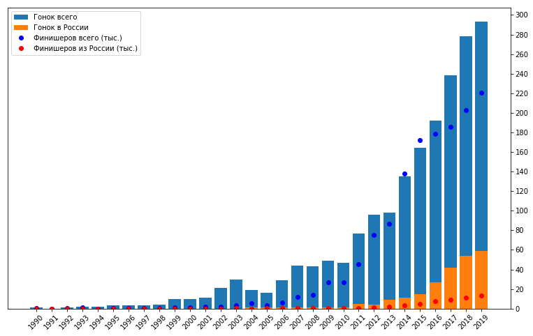 It can be seen that the number of races and participants at the beginning of the period and at the end is simply incommensurable. A significant increase in the total number of races begins in 2011, while the number of starts in Russia also increases. Moreover, an increase in the number of participants can be observed back in 2009. This may indicate increased interest among the participants, that is, increased demand, after which two years later supply increased, that is, the number of starts. However, do not forget that the data may not be complete and some, and possibly many races are missing. Including due to the fact that the project to collect this data began only in 2010, which can also explain the significant leap in the graph at this very moment. Including therefore, for further analysis, I decided to take the last 10 years. This is a fairly long period,in order to track any trends over several years, while short enough to not get there, mainly professional competitions from the 90s and early 2000s.
rs = rs[(rs['year']>=2010)&(rs['year']<= 2019)]
 In the selected period, by the way, 84% of races and 94% of finishers fell.
Amateur starts
So, the vast majority of participants in the selected starts are amateur athletes, so good statistics can be obtained from them. Honestly, this was of main interest to me, since I myself participate in such starts, but in level it is very far from the Olympic champions. However, professional competitions obviously also took place in the selected period. In order not to mix the indicators for amateur and professional races, it was decided to remove the latter from consideration. How to identify them? By speed. We calculate them. At one of the initial stages of data preparation, we already determined what type of distance was on each race - sprint, Olympic, half, iron. For each of them, the mileage of the stages is clearly defined - swimming, cycling and running. This is 0.75 + 20 + 5 for the sprint, 1.5 + 40 + 10 for the Olympic, 1.9 + 90 + 21.1 for the half and 3.8 + 180 + 42.2 for iron. Of course, in fact, for any type, real numbers can vary from race to race conditionally up to one percent, but there is no information about this, so we will assume that everything was accurate.rs['km'] = ''
rs.loc[rs['dist'] == 'sprint', 'km'] = 0.75+20+5
rs.loc[rs['dist'] == 'olympic', 'km'] = 1.5+40+10
rs.loc[rs['dist'] == 'half', 'km'] = 1.9+90+21.1
rs.loc[rs['dist'] == 'full', 'km'] = 3.8+180+42.2
We calculate the average and maximum speeds for each race. The maximum here refers to the average speed of the athlete who won first place.for index, row in rs.iterrows():
e = row['event']
rd[e]['th'] = pd.TimedeltaIndex(rd[e]['result']).seconds/3600
rd[e]['v'] = rs.loc[i, 'km'] / rd[e]['th']
for index, row in rs.iterrows():
e = row['event']
rs.loc[index,'vmax'] = rd[e]['v'].max()
rs.loc[index,'vavg'] = rd[e]['v'].mean()
 Well, you can see that the bulk of the speeds gathered in heaps between about 15 km / h and 30 km / h, but there are a certain number of completely "cosmic" values. Sort by average speed and see how many of them:
rs = rs.sort_values(by='vavg')
 Here we changed the scale and we can estimate the range more accurately. For average speeds it is from about 17 km / h to 27 km / h, for maximum - from 18 km / h to 32 km / h. Plus there are “tails” with very low and very high average speeds. Low speeds most likely correspond to extreme competitions like Norseman , and high speeds can be in the case of canceled swimming, where instead of a sprint there was a super sprint, or simply erroneous data. Another important point is the smooth step in the 1200 area along the X axis, and higher values of the average speed after it. There you can see a significantly smaller difference between the average and maximum speeds than in the first two-thirds of the graph. Apparently, this is a professional competition. To distinguish them more clearly, we calculate the ratio of maximum speed to average. In professional competitions where there are no random people and all participants have a very high level of physical fitness, this ratio should be minimal.
rs['vmdbva'] = rs['vmax']/rs['vavg']
rs = rs.sort_values(by='vmdbva')
 On this graph, the first quarter stands out very clearly: the ratio of maximum speed to average is small, high average speed, a small number of participants. This is a professional competition. The step on the green curve is somewhere around 1.2. We will leave only records with a ratio value greater than 1.2 in our sample.
rs = rs[rs['vmdbva'] > 1.2]
We also remove records with atypical low and high speeds. In What are the triathlon “world records” for each distance? published record times of passing different distances for 2019. If you count them at medium speeds, you can see that it can not be higher than 33 km / h even for the fastest. So we will consider the protocols where the average speeds are higher, invalid, and remove them from consideration.rs = rs[(rs['vavg'] > 17)&(rs['vmax'] < 33)]
Here's what remains:
 Now everything looks quite homogeneous and does not raise questions. As a result of all this selection, we lost 777 of the 1922 protocols, or 40%. At the same time, the total number of finishers did not decrease so much - by only 13%.So, there are 1,145 races left with 1,231,772 finishers. This sample became the material for my analysis and visualization.
Part 5. Analysis and visualization
In this work, analysis and visualization proper were the simplest parts. The tip of the iceberg, the underwater part of which was just the preparation of the data. The analysis, in fact, was a simple arithmetic operation on the pandas Series , calculating averages, filtering - all this is done by the elementary pandas tools and the above code is full of examples. Visualization, in turn, was mainly done using the most standard matplotlib . Used plot, bar, pie . In some places, however, I had to tinker with the signatures of the axes, in the case of dates and pictograms, but this is not something that draws on a detailed description here. The only thing worth talking about is the presentation of geodata. At least it's notmatplotlib .Geodata
For each race we have information about the venue. At the very beginning, using geopy, we calculated the coordinates for each location. Many races are held annually in the same place. A very handy tool for rendering geodata in python is folium . Here's how it works:import folium
m = folium.Map()
folium.Marker(['55.7522200', '37.6155600'], popup='').add_to(m)
And we get an interactive map right in the Jupiter laptop. Now, to our data. First, we’ll start a new column from a combination of our coordinates:
rs['coords'] = rs['latitude'].astype(str) + ', ' + rs['longitude'].astype(str)
The unique coordinates of coords are 291. And the unique locations loc are 324, which means that some names differ slightly, while at the same time they correspond to the same point. It's not scary, we will consider uniqueness by coords . We calculate how many events have passed over the entire time in each location (with unique coordinates):vc = rs['coords'].value_counts()
vc
Out:
43.7009358, 7.2683912 22
43.5854823, 39.723109 20
29.03970805, -13.636291 16
47.3723941, 8.5423328 16
59.3110918, 24.420907 15
51.0834196, 10.4234469 15
54.7585694, 38.8818137 14
20.4317585, -86.9202745 13
52.3727598, 4.8936041 12
41.6132925, 2.6576102 12
... ...
Now create a map, and add markers on it in the form of circles, the radius of which will depend on the number of events held on the location. Add markers with location name to the markers.m = folium.Map(location=[25,10], zoom_start=2)
for c in rs['coords'].unique():
row = [r[1] for r in rs.iterrows() if r[1]['coords'] == c][0]
folium.Circle([row['latitude'], row['longitude']],
popup=(row['location']+'\n('+str(vc[c])+' races)'),
radius = 10000*int(vc[c]),
color='darkorange',
fill=True,
stroke=True,
weight=1).add_to(m)
Done. You can see the result:
Participants Progress
In fact, in addition to guiding, work on yet another schedule was also non-trivial. This is the latest progress graph of participants. Here it is: Let's analyze it, at the same time I will give the code for rendering, as an example of using matplotlib :
fig = plt.figure()
fig.set_size_inches(10, 6)

ax = fig.add_axes([0,0,1,1])

b = ax.bar(exp,numrecs, color = 'navajowhite')

ax1 = ax.twinx()

for i in range(len(exp_samp)):
    ax1.plot(exp_samp[i], vproc_samp[i], '.')

p, = ax1.plot(exp, vpm, 'o-',markersize=8, linewidth=2, color='C0')

for i in range(len(exp)):
    if i < len(exp)-1 and (vpm[i] < vpm[i+1]):
        ax1.text(x = exp[i]+0.1, y = vpm[i]-0.2, s = '{0:3.1f}%'.format(vpm[i]),size=12)
    else:
        ax1.text(x = exp[i]+0.1, y = vpm[i]+0.1, s = '{0:3.1f}%'.format(vpm[i]),size=12)

ax.legend((b,p), (' ', ''),loc='center right')
ax.set_xlabel('   ')
ax.set_ylabel('')
ax1.set_ylabel('%     ')
ax.set_xticks(np.arange(1, 11, step=1))
ax.set_yticks(np.arange(0, 230000, step=25000))
ax1.set_ylim(97.5,103.5)
ax.yaxis.set_label_position("right")
ax.yaxis.tick_right()
ax1.yaxis.set_label_position("left")
ax1.yaxis.tick_left()

plt.show()
Now about how the data was calculated for him. First, you had to choose the names of the participants who finished at least in two races, and in different calendar years, and at the same time are not professionals.First, for each protocol, fill in a new column called date , which will indicate the date of the race. We will also need a year from this date, we will make the column year . Since we are going to analyze the speed of each athlete relative to the average speed in the race, we immediately calculate this speed in the new column vproc - the speed as a percentage of the average.for index, row in rs.iterrows():
e = row['event']
rd[e]['date'] = row['date']
rd[e]['year'] = row['year']
rd[e]['vproc'] = 100 * rd[e]['v'] / rd[e]['v'].mean()
Here's what the protocols now look like: Next, combine all the protocols into a single data frame.' Sprint 2019'ar = pd.concat(rd)
For each participant, we will leave only one entry in each calendar year:ar1 = ar.drop_duplicates(subset = ['name','year'], keep='first')
Next, from all the unique names of these entries, we find those that occur at least twice:nvc = ar1['name'].value_counts()
names = list(nvc[nvc > 1].index)
there are 219,890 of them. Let's remove the names of pro-athletes from this list:pro_names = ar[ar['group'].isin(['MPRO','FPRO'])]['name'].unique()
names = list(set(names) - set(pro_names))
As well as the names of athletes who began performing before 2010. To do this, upload the data that was saved before we sampled in the last 10 years. Put them in the rsa (races summary all) and rda (race details all) objects .rdo = {}
for e in rda:
if rsa[rsa['event'] == e]['year'].iloc[0] < 2010:
rdo[e] = rda[e]
aro = pd.concat(rdo)
old_names = aro['name'].unique()
names = list(set(names) - set(old_names))
And finally, we find names that occur more than once on the same day. Thus, we minimize the presence of full namesakes in our sample.namesakes = ar[ar.duplicated(subset = ['name','date'], keep = False)]['name'].unique()
names = list(set(names) - set(namesakes))
So there are 198,075 names left. From the entire dataset, we select only the records with the names found:ars = ar[ar['name'].isin(names)]
Now, for each record, you need to determine which year in the athlete’s career it corresponds to - the first, second, third, or tenth. We make a loop by all names and calculate.ars['exp'] = ''
for n in names:
ind = ars[ars['name'] == n].index
yos = ars.loc[ind, 'year'].min()
ars.loc[ind, 'exp'] = ars.loc[ind, 'year'] - yos + 1
Here is an example of what happened: Apparently, the namesakes still remained. This is expected, but not scary, as we will average everything, and there should not be so many. Next, we build arrays for the graph:exp = []
vpm = []
numrecs = []
for x in range(ars['exp'].min(), ars['exp'].max() + 1):
exp.append(x)
vpm.append(ars[ars['exp'] == x]['vproc'].mean())
numrecs.append(len(ars[ars['exp'] == x]))
That's it, there is a basis: Now, to decorate it with points that correspond to specific results, we will select 1000 random names and build arrays with the results for them.
names_samp = random.sample(names,1000)
ars_samp = ars[ars['name'].isin(names_samp)]

ars_samp = ars_samp.reset_index(drop = True)
exp_samp = []
vproc_samp = []

for n in names_samp:
    nr = ars_samp[ars_samp['name'] == n]
    nr = nr.sort_values('exp')
    exp_samp.append(list(nr['exp']))
    vproc_samp.append(list(nr['vproc']))
Add a loop to build graphs from this random sample.for i in range(len(exp_samp)):
ax1.plot(exp_samp[i], vproc_samp[i], '.')
Now everything is ready: In general, it is not difficult. But there is one problem. To calculate the exp experience in a cycle, all names, which are almost 200 thousand, take eight hours. I had to debug the algorithm on small samples, and then run the calculation for the night. In principle, this can be done once, but if you find some kind of error or want to change something, and you need to recount it again, it starts to strain. And so, when I was going to publish a report in the evening, it turned out that again it was necessary to recount everything again. Waiting until morning was not part of my plans, and I began to look for a way to make the calculation faster. Decided to parallelize.Found somewhere a way to do this with multiprocessing. In order to work on Windows, we needed to put the main logic of each parallel task into a separate workers.py file:
import pickle as pkl

def worker(args):
    names = args[0]
    ars=args[1]
    num=args[2]
    ars = ars.sort_values(by='name')
    ars = ars.reset_index(drop=True)

    for n in names:
        ind = ars[ars['name'] == n].index
        yos = ars.loc[ind, 'year'].min()
        ars.loc[ind, 'exp'] = ars.loc[ind, 'year'] - yos + 1

    with open(r'D:\tri\par\prog' + str(num) + '.pkl', 'wb') as f:
        pkl.dump(ars,f)
The procedure is transferred to a portion of the names of names , part datafreyma ar only with these names, and the serial number of parallel tasks - num . Computations are written to the data frame and, at the end, the data frame is written to the file. In the laptop that calls this worker , we prepare the arguments accordingly:num_proc = 8
args = []
for i in range(num_proc):
step = int(len(names_samp)/num_proc) + 1
names_i = names_samp[i*step:min((i+1)*step, len(names_samp))]
ars_i = ars[ars['name'].isin(names_i)]
args.append([names_i, ars_i, i])
We start parallel computing:from multiprocessing import Pool
import workers
if __name__ == '__main__':
p=Pool(processes = num_proc)
p.map(workers.worker,args)
And at the end we read the results from the files and collect the pieces back into the whole data frame:ars=pd.DataFrame(columns = ars.columns)
for i in range(num_proc):
with open(r'D:\tri\par\prog'+str(i)+'.pkl', 'rb') as f:
arsi = pkl.load(f)
print(len(arsi))
ars = pd.concat([ars, arsi])
Thus, it was possible to obtain an acceleration of 40 times, and instead of 8 hours to complete the calculation in 11 minutes and publish a report that evening. At the same time I learned how to parallelize in python , I think it will come in handy. Here, the acceleration turned out to be even more than just 8 times the number of cores, due to the fact that each task used a small data frame, which makes searching faster. In principle, sequential calculations could be accelerated in this way, but the question is, how do you guess?However, I could not calm down and even after the publication I was constantly thinking about how to do the calculation using vectorization, that is, operations on whole columns of the pandas Series data frame. Such calculations are an order of magnitude faster than any parallelized cycles, even on a supercluster. And came up with. It turns out that for each name to find the year of the beginning of a career, it is necessary on the contrary - for each year to find the participants who started in it. To do this, you must first determine all the names for the first year from our sample, this is 2010. Accordingly, we process all records with these names using this year. Next, we take the next year - 2011.Again we find all the names with entries this year, but we take from them only unprocessed ones, that is, those that were not met in 2010 and are processed using them in 2011. And so on for the rest of the year. The same cycle, but not two hundred thousand iterations, but nine in total.for y in range(ars['year'].min(),ars['year'].max()):
arsynp = ars[(ars['exp'] == '') & (ars['year'] == y)]
namesy = arsynp['name'].unique()
ind = ars[ars['name'].isin(namesy)].index
ars.loc[ind, 'exp'] = ars.loc[ind,'year'] - y + 1
This cycle fulfills in just a couple of seconds. And the code turned out to be much more concise.Conclusion
Well, finally, a lot of work has been completed. For me, this was, in fact, the first project of its kind. When I took it, the main goal was to practice using python and its libraries. This task is more than completed. And the results themselves were quite presentable. What conclusions did I draw for myself upon completion?First: Data is imperfect. This is probably true for almost any analysis task. Even if they are completely structured, and it often happens differently, you need to be prepared to tinker with them before you start calculating the characteristics and searching for trends - find errors, outliers, deviations from standards, etc.Second:Any task has a solution. This is more like a slogan, but often it is. It’s just that this solution may not be so obvious and does not lie in the data itself, but outside of the box, so to speak. As an example - the processing of the names of participants described above, or website scraping.Third: Domain knowledge is crucial. This will make it possible to better prepare the data, removing obviously invalid or non-standard data, avoid interpretation errors, use information that is not in the data, for example, distances in this project, present the results in the form accepted in the community, while avoiding stupid, incorrect conclusions.Fourth: To work in pythonThere is a rich set of tools. Sometimes it seems that it is worth thinking about something, you begin to search - it already exists. This is just great! Many thanks to the creators for this contribution, especially for the tools that came in handy here: selenium for scraping, pycountry for determining the country code according to the ISO standard, country codes (datahub) for Olympic codes, geopy for determining the coordinates at the address, folium - for visualization of geodata, gender-guesser - for the analysis of names, multiprocessing - for parallel computing, matplotlib , numpy , and of course pandas - without it there’s nowhere to go.Fifth: Vectorization is our everything. It is extremely important to be able to use the built-in pandas tools , it is very effective. I suppose, in most cases, when the number of records is measured starting from tens of thousands, this skill becomes simply necessary.Sixth:Handling data is a bad idea. It is necessary to try to minimize any manual intervention - firstly, it does not scale, that is, when the amount of data increases several times, the time for manual processing will increase to unacceptable values, and secondly, there will be poor repeatability - you will forget something, you will make a mistake somewhere . Everything is only programmatic, if something falls out of the general standard for a software solution, well, it's okay, you can sacrifice some part of the data, there will still be more pluses.Seventh:The code must be kept in working order. It would seem that it could be more obvious! In fact, when it comes to code for your own use, the purpose of which is to publish the results of this code, everything is not so strict here. I worked in Jupiter Notebooks, and this environment, in my opinion, just does not have to create integral software products. It is configured for line-by-line, piecewise launch, this has its advantages - it is fast: development, debugging and execution at the same time. But often the temptation is to just edit some line and quickly get a new result, instead of duplicating or wrapping in def. Of course, such a temptation should be avoided. One should strive for a good code, even “for oneself”, at least because even for one analysis work the launch is done many times, and investing time in the beginning will surely pay off in the future. And you can add tests, even on laptops, in the form of checks of critical parameters and throwing exceptions - it is very useful.Eighth: Save more often. At each step, I saved a new version of the file. In total, they turned out to be about 10. This is convenient, since when an error is detected it helps to quickly determine at what stage it occurred. Plus, I saved the source data in the columns marked raw - this allows you to quickly check the result and see the discrepancy.Ninth:It is necessary to measure the investment of time and the result. In some places, I took a very long time to restore data, which form a fraction of a percent of the total. In fact, this made no sense, you just had to throw them away, and that’s all. And I would do so if it were a commercial project, not an auto-training. This would allow you to get the result much faster. The Pareto principle works here - 80% of the result is achieved in 20% of the time.And the last one:Work on such projects greatly broadens the horizons. Willingly, you learn something new - for example, the names of strange countries - such as the Pitcairn Islands, that the ISO code for Switzerland is CHE, from the Latin “Confoederatio Helvetica”, what is the Spanish name, well, actually about the triathlon itself - records, their owners, places of races, history of events and so on.Perhaps enough. That's all. Thanks to everyone who read to the end!