👨🏼‍🚒 🚰 🌏 Concurrency, coroutines, event machines, ... living math 🙎🏿 📈 🤞🏽

Parallel computing fascinates with the unexpectedness of its behavior. But the joint behavior of processes cannot be unpredictable. Only in this case can he be studied and understood in his quirks. Modern multi-threaded concurrency is unique. In a literal sense. And this is all his ~~bad~~ essence. The essence that can and should be influenced. The essence, which should, in a good way, have long been changed ...

Although there is another option. There is no need to change anything and / or influence something. Let there be multithreading and coroutines, let it be ... and parallel automatic programming (AP). Let them compete and, when necessary and possible, complement each other. In this sense, modern parallelism has at least one plus - it allows you to do this.

~~Well, let's compete !?~~

1. From serial to parallel

Consider programming the simplest arithmetic equation:

C2 = A + B + A1 + B1; (1)

Let there be blocks that implement simple arithmetic operations. In this case, summing blocks are sufficient. A clear and accurate idea of the number of blocks, their structure and the relationships between them gives rice. 1. And in Fig. 2. the configuration of the VKP (a) medium is given for solving equation (1).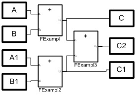

Fig. 1. Structural model of processes

But the structural diagram in Fig. 1 corresponds to a system of three equations:

= A + B;
C1 = A1 + B; (2)
C2 = C + C1;

At the same time (2), this is a parallel implementation of equation (1), which is an algorithm for summing an array of numbers, also known as a doubling algorithm. Here the array is represented by four numbers A, B, A1, B1, variables C and C1 are intermediate results, and C2 is the sum of the array.

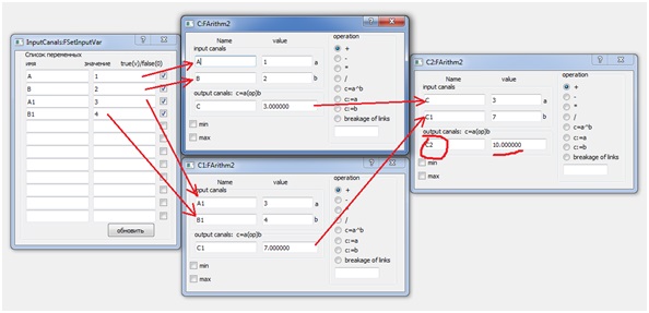Fig. 2. Type of dialogs for the configuration of three parallel processes.

The implementation features include the continuity of its operation, when any change in the input data leads to a recount of the result. After changing the input data, it will take two clock cycles, and when the blocks are connected in series, the same effect will be achieved in three clock cycles. And the larger the array, the greater the speed gain.

2. Concurrency as a problem

Do not be surprised if you will be called many arguments in favor of one or another parallel solution, but at the same time they will be silent about possible problems that are completely absent in ordinary sequential programming. The main reason for the similar interpretation of the problem of the correct implementation of parallelism. They say the least about her. If at all they say. We will touch upon it in the part related to parallel access to data.

Any process can be represented as many consecutive indivisible steps. For many processes, at each such step, actions belonging to all processes are executed simultaneously. And here we may well encounter a problem that manifests itself in the following elementary example.

Suppose there are two parallel processes that correspond to the following system of equations:

c = a + b; (3)
a = b + c;

Suppose the variables a, b, c are assigned the initial values 1, 1, 0. We can expect that the calculation protocol for the five steps will be as follows:

a              b               c
1.000       1.000       0.000      
1.000       1.000       2.000       
3.000       1.000       2.000       
3.000       1.000       4.000       
5.000       1.000       4.000        
5.000       1.000       6.000

When forming it, we proceeded from the fact that the operators are executed in parallel (simultaneously) and within one discrete measure (step). For looped statements, it will be an iteration of the loop. We can also assume that in the process of calculations the variables have values fixed at the beginning of a discrete measure, and their change occurs at its end. This is quite consistent with the real situation, when it takes some time to complete the operation. It is often associated with a delay inherent in a given block.

But, most likely, you will get something like this protocol:

   a              b               c
1.000       1.000       0.000      
3.000       1.000       2.000       
5.000       1.000       4.000       
7.000       1.000       6.000       
9.000       1.000       8.000       
11.000     1.000     10.000

It is equivalent to the work of a process executing two consecutive statements in a cycle:

c = a + b; a = b + c; (4)

But it may happen that the execution of the statements will be exactly the opposite, and then the protocol will be as follows:

   a              b               c
1.000       1.000       0.000      
1.000       1.000       2.000       
3.000       1.000       4.000       
5.000       1.000       6.000       
7.000       1.000       8.000       
9.000       1.000     10.000

In multi-threaded programming, the situation is even worse. In the absence of synchronization of processes, it is not only difficult to predict the sequence of operators launching, but their work will also be interrupted anywhere. All this cannot but affect the results of the joint work of the operators.

Within the framework of AP technology, work with common process variables is allowed simply and correctly. Here, most often, no special efforts are required to synchronize processes and work with data. But it will be necessary to single out actions that will be considered conditionally instantaneous and indivisible, as well as create automatic process models. In our case, the actions will be summation operators, and automata with cyclic transitions will be responsible for their launch.
Listing 1 shows the code for a process that implements the sum operation. Its model is a finite state machine (see Fig. 3) with one state and an unconditional loop transition, for which the only action y1, having performed the operation of summing two variables, puts the result in the third.

Fig. 3. Automated model of the operation of summation

Listing 1. Implementation of an automaton process for a sum operation

#include "lfsaappl.h"
class FSumABC :
    public LFsaAppl
{
public:
    LFsaAppl* Create(CVarFSA *pCVF) { Q_UNUSED(pCVF)return new FSumABC(nameFsa); }
    bool FCreationOfLinksForVariables();
    FSumABC(string strNam);
    CVar *pVarA;		//
    CVar *pVarB;		//
    CVar *pVarC;		//
    CVar *pVarStrNameA;        //
    CVar *pVarStrNameB;        //
    CVar *pVarStrNameC;        //
protected:
    void y1();
};

#include "stdafx.h"
#include "FSumABC.h"

static LArc TBL_SumABC[] = {
    LArc("s1",	"s1","--", "y1"),
    LArc()
};

FSumABC::FSumABC(string strNam):
    LFsaAppl(TBL_SumABC, strNam, nullptr, nullptr)
{ }

bool FSumABC::FCreationOfLinksForVariables() {
    pVarA = CreateLocVar("a", CLocVar::vtBool, "variable a");
    pVarB = CreateLocVar("b", CLocVar::vtBool, "variable c");
    pVarC = CreateLocVar("c", CLocVar::vtBool, "variable c");
    pVarStrNameA = CreateLocVar("strNameA", CLocVar::vtString, "");
    string str = pVarStrNameA->strGetDataSrc();
    if (str != "") { pVarA = pTAppCore->GetAddressVar(pVarStrNameA->strGetDataSrc().c_str(), this); }
    pVarStrNameB = CreateLocVar("strNameB", CLocVar::vtString, "");
    str = pVarStrNameB->strGetDataSrc();
    if (str != "") { pVarB = pTAppCore->GetAddressVar(pVarStrNameB->strGetDataSrc().c_str(), this); }
    pVarStrNameC = CreateLocVar("strNameC", CLocVar::vtString, "");
    str = pVarStrNameC->strGetDataSrc();
    if (str != "") { pVarC = pTAppCore->GetAddressVar(pVarStrNameC->strGetDataSrc().c_str(), this); }
    return true;
}

void FSumABC::y1() { 
    pVarC->SetDataSrc(this, pVarA->GetDataSrc() + pVarB->GetDataSrc()); 
}

Important, or rather, even necessary, here is the use of the environment variables of the CPSU. Their “shadow properties” ensure the correct interaction of processes. Moreover, the environment allows you to change the mode of its operation, excluding the recording of variables in the intermediate shadow memory. An analysis of the protocols obtained in this mode allows us to verify the necessity of using shadow variables.

3. And the coroutines? ...

It would be nice to know how the coroutines represented by the Kotlin language will cope with the task. Let us take as a solution template the program considered in the discussion of [1]. It has a structure that is easily reduced to the required look. To do this, replace the logical variables in it with a numeric type and add another variable, and instead of logical operations we will use the summation operation. The corresponding code is shown in listing 2.

Listing 2. Kotlin parallel summation program

import kotlinx.coroutines.*

suspend fun main() =
    // Structured concurrency: if any child coroutine fails,
    // everything else will be cancelled
    coroutineScope {
        var a = 1
        var b = 1
        var c = 0;
        // Use default thread pool 
        withContext(Dispatchers.Default) {
            for (i in 0..4) {
               var res = listOf(async { a+b }, async{ b+c }).map { it.await() }
			c = res[0]
			a = res[1]
               println("$a, $b, $c")
            }
        }
    }

There are no questions about the result of this program, as it exactly matches the first of the above protocols.

However, the conversion of the source code was not as obvious as it might seem, because It seemed natural to use the following code fragment:

listOf(async {  = a+b }, async{  = b+c })

As shown by testing (this can be done online on the Kotlin website - kotlinlang.org/#try-kotlin ), its use leads to a completely unpredictable result, which also changes from launch to launch. And only a more careful analysis of the source program led to the correct code.

Code that contains an error from the point of view of the functioning of the program, but is legitimate from the point of view of the language, makes us fear for the reliability of the programs on it. This opinion, probably, can be challenged by Kotlin experts. Nevertheless, the ease of making a mistake, which cannot be explained only by a lack of understanding of “coroutine programming,” is nevertheless persistently pushing for such conclusions.

4. Event machines in Qt

Earlier, we established that an event automaton is not an automaton in its classical definition. He is good or bad, but to some extent the event machine is still a relative of classical machines. Is it distant, near, but we must talk about it directly so that there are no misconceptions about this. We started talking about this in [2], but all for continuing it. Now we will do this by examining other examples of the use of event machines in Qt.

Of course, an event automaton can be considered as a degenerate case of a classical automaton with an indefinite and / or variable cycle duration associated with an event. The possibility of such an interpretation was shown in a previous article when solving only one and, moreover, a rather specific example (see details [2]). Next, we will try to eliminate this gap.

The Qt library only associates machine transitions with events, which is a serious limitation. For example, in the same UML language, a transition is associated not only with an event called an initiating event, but also with a protective condition - a logical expression calculated after the event is received [3]. In MATLAB, the situation is mitigated more and sounds like this: “if the name of the event is not specified, then the transition will occur when any event occurs” [4]. But here and there, the root cause of the transition is the event / s. But what if there are no events?

If there are no events, then ... you can try to create them. Listing 3 and Figure 4 demonstrate how to do this, using the descendant of the automaton class LFsaAppl of the VKPa environment as a "wrapper" of the event Qt-class. Here, the action y2 with a periodicity of the discrete time of the automaton space sends a signal initiating the start of the transition of the Qt automaton. The latter, using the s0Exited method, starts the action y1, which implements the summation operation. Note that the event machine is created by the action y3 strictly after checking the initialization of local variables of the LFsaAppl class.

Fig. 4. Combination of classic and event machines

Listing 3. Implementing a summation model with an event automaton

#include "lfsaappl.h"
class QStateMachine;
class QState;

class FSumABC :
    public QObject,
    public LFsaAppl
{
    Q_OBJECT
...
protected:
    int x1();
    void y1(); void y2(); void y3(); void y12();
signals:
    void GoState();
private slots:
    void s0Exited();
private:
    QStateMachine * machine;
    QState * s0;
};

#include "stdafx.h"
#include "FSumABC.h"
#include <QStateMachine>
#include <QState>

static LArc TBL_SumABC[] = {
    LArc("st",	"st","^x1",	"y12"),
    LArc("st",	"s1","x1",	"y3"),
    LArc("s1",	"s1","--",	"y2"),
    LArc()
};

FSumABC::FSumABC(string strNam):
    QObject(),
    LFsaAppl(TBL_SumABC, strNam, nullptr, nullptr)
{ }
...
int FSumABC::x1() { return pVarA&&pVarB&&pVarC; }

void FSumABC::y1() {
    pVarC->SetDataSrc(this, pVarA->GetDataSrc() + pVarB->GetDataSrc());
}
//
void FSumABC::y2() { emit GoState(); }
//
void FSumABC::y3() {
    s0 = new QState();
    QSignalTransition *ps = s0->addTransition(this, SIGNAL(GoState()), s0);
    connect (s0, SIGNAL(entered()), this, SLOT(s0Exited()));
    machine = new QStateMachine(nullptr);
    machine->addState(s0);
    machine->setInitialState(s0);
    machine->start();
}
//    
void FSumABC::y12() { FInit(); }

void FSumABC::s0Exited() { y1(); }

Above, we implemented a very simple machine. Or, more precisely, a combination of classic and event automatons. If the previous implementation of the FSumABC class is replaced with the created one, then there will simply be no differences in the application. But for more complex models, the limited properties of event-driven automata begin to fully manifest themselves. At a minimum, already in the process of creating a model. Listing 4 shows the implementation of the model of the AND-NOT element in the form of an event automaton (for more details on the used automaton model of the AND-NOT element, see [2]).

Listing 4. Implementing an element model AND NOT by an event machine

#include <QObject>

class QStateMachine;
class QState;

class MainWindow;
class ine : public QObject
{
    Q_OBJECT
public:
    explicit ine(MainWindow *parent = nullptr);
    bool bX1, bX2, bY;
signals:
    void GoS0();
    void GoS1();
private slots:
    void s1Exited();
    void s0Exited();
private:
    QStateMachine * machine;
    QState * s0;
    QState * s1;
    MainWindow *pMain{nullptr};
friend class MainWindow;
};

#include "ine.h"
#include <QStateMachine>
#include <QState>
#include "mainwindow.h"
#include "ui_mainwindow.h"

ine::ine(MainWindow *parent) :
    QObject(parent)
{
    pMain = parent;
    s0 = new QState();
    s1 = new QState();

    s0->addTransition(this, SIGNAL(GoS1()), s1);
    s1->addTransition(this, SIGNAL(GoS0()), s0);

    connect (s0, SIGNAL(entered()), this, SLOT(s0Exited()));
    connect (s1, SIGNAL(entered()), this, SLOT(s1Exited()));


    machine = new QStateMachine(nullptr);
    machine->addState(s0);
    machine->addState(s1);
    machine->setInitialState(s1);
    machine->start();
}

void ine::s1Exited() {
    bY = !(bX1&&bX2);
    pMain->ui->checkBoxY->setChecked(bY);
}

void ine::s0Exited() {
    bY = !(bX1&&bX2);
    pMain->ui->checkBoxY->setChecked(bY);
}

It becomes clear that event automata in Qt are based strictly on Moore automata. This limits the capabilities and flexibility of the model, as actions are associated only with states. As a result, for example, it is impossible to distinguish between two transitions from the 0 to 1 state for the automaton shown in Fig. 4 in [2].

Of course, to implement the Miles, you can use the well-known procedure for switching to Moore machines. But this leads to an increase in the number of states and eliminates the simple, visual and useful association of model states with the result of its actions. For example, after such transformations, the two states of the Moore automaton must be matched to the single state of the output of model 1 from [2].

On a more complex model, problems with transition conditions begin to appear with obviousness. To get around them for the software implementation of the AND-NOT element under consideration, an analysis of the state of the input channels was built into the model control dialog, as shown in Listing 5.

Listing 5. NAND element control dialog

#include "mainwindow.h"
#include "ui_mainwindow.h"
#include "ine.h"

MainWindow::MainWindow(QWidget *parent)
    : QMainWindow(parent)
    , ui(new Ui::MainWindow)
{
    ui->setupUi(this);
    pine = new ine(this);
    connect(this, SIGNAL(GoState0()), pine, SIGNAL(GoS0()));
    connect(this, SIGNAL(GoState1()), pine, SIGNAL(GoS1()));
}

MainWindow::~MainWindow()
{
    delete ui;
}


void MainWindow::on_checkBoxX1_clicked(bool checked)
{
    bX1 = checked;
    pine->bX1 = bX1;
    bY = !(bX1&&bX2);
    if (!(bX1&&bX2)) emit GoState0();
    else emit GoState1();
}

void MainWindow::on_checkBoxX2_clicked(bool checked)
{
    bX2 = checked;
    pine->bX2 = bX2;
    bY = !(bX1&&bX2);
    if (!(bX1&&bX2)) emit GoState0();
    else emit GoState1();
}

In sum, all of the above clearly complicates the model and creates problems with understanding its work. In addition, such local solutions may not work when considering compositions from them. A good example in this case would be an attempt to create an RS-trigger model (for more details on a two-component automaton model of an RS-trigger see [5]). However, the pleasure of the achieved result will be delivered to fans of event machines. If ... unless, of course, they succeed;)

5. Quadratic function and ... butterfly?

It is convenient to represent the input data as an external parallel process. Above this was the dialog for managing the model of an AND-NOT element. Moreover, the rate of change of data can significantly affect the result. To confirm this, we consider the calculation of the quadratic function y = ax² + bx + c, which we implement in the form of a set of parallel-functioning and interacting blocks.

The graph of a quadratic function is known to have the shape of a parabola. But the parabola depicted by the mathematician and the parabola that the oscilloscope, for example, will display, strictly speaking, will never match. The reason for this is that the mathematician often thinks in instantaneous categories, believing that a change in the input quantity leads immediately to the calculation of the function. But in real life this is not at all true. The appearance of the function graph will depend on the speed of the calculator, on the rate of change of the input data, etc. etc. Yes, and the programs themselves for speed may differ from each other. These factors will affect the form of the function, in the form of which in a certain situation it will be difficult to guess the parabola. We will be convinced of this further.

So, we add to the summing block the blocks of multiplication, division and exponentiation. Having such a set, we can “collect” mathematical expressions of any complexity. But we can also have “cubes” that implement more complex functions. Fig. 5. implementation of a quadratic function is shown in two versions - multi-block (see arrow with a label - 1, and also Fig. 6) and a variant from one block (in Fig. 5 arrow with a label 2).

Fig.5. Two options for implementing the quadratic function

Fig. 6. Structural model for calculating a quadratic function

That in fig. 5. it seems “blurred” (see arrow marked 3), when properly enlarged (see graphs (trends), marked 4), it is convinced that the matter is not in the graphics properties. This is the result of the influence of time on the calculation of variables: the variable y1 is the output value of the multi-block variant (red color of the graph) and the variable y2 is the output value of the single-block variant (black color). But both of these graphics are different from the "abstract graphics" [y2 (t), x (t-1)] (green). The latter is constructed for the value of the variable y2 and the value of the input variable delayed by one clock cycle (see the variable with the name x [t-1]).

Thus, the higher the rate of change of the input function x (t), the stronger the “blurring effect” will be and the farther the graphs y1, y2 will be from the graph [y2 (t), x (t-1)]. The detected "defect" can be used for your own purposes. For example, nothing prevents us from applying a sinusoidal signal to the input. We will consider an even more complicated option, when the first coefficient of the equation also changes in a similar way. The result of the experiment demonstrates a screen of the VKPa medium, shown in Fig. 7.

Fig. 7. Simulation results with a sinusoidal input signal

The screen on the lower left shows the signal supplied to the inputs of realizations of a quadratic function. Above it are the graphs of the output values y1 and y2. Charts in the form of “wings” are values plotted in two coordinates. So, with the help of various realizations of the quadratic function, we drew the half of the “butterfly”. To draw a whole is a matter of technology ...

But the paradoxes of parallelism do not end there. In fig. Figure 8 shows trends in the “reverse” change of the independent variable x. They pass already to the left of the "abstract" graph (the latter, we note, has not changed its position!).

Fig. 8. The type of graphs with direct and reverse linear change of the input signal

In this example, the “double” error of the output signal with respect to its “instantaneous” value becomes apparent. And the slower the computing system or the higher the signal frequency, the greater the error. A sine wave is an example of a forward and reverse change of an input signal. Due to this, the “wings” in Fig. 4 took this form. Without the “backward error” effect, they would be twice as narrow.

6. Adaptive PID Controller

Let's consider one more example on which the considered problems are shown. In fig. Figure 9 shows the configuration of the VKP (a) medium when modeling an adaptive PID controller. A block diagram is also shown in which the PID controller is represented by a unit named PID. At the black box level, it is similar to the previously considered single-block implementation of a quadratic function.

The result of comparing the results of the calculation of the PID controller model within a certain mathematical package and the protocol obtained from the simulation results in the VKP (a) environment is shown in Fig. 10, where the red graph is the calculated values, and the blue graph is the protocol. The reason for their mismatch is that the calculation within the framework of the mathematical package, as shown by further analysis, corresponds to the sequential operation of the objects when they first work out the PID controller and stop, and then the model of the object, etc. in the loop. The VKPa environment implements / models the parallel operation of objects according to the real situation, when the model and the object work in parallel.

Fig. 9. Implementation of the PID controller

Fig. 10. Comparison of calculated values with simulation results of the PID controller

Since, as we already announced, VKP (a) has a mode for simulating the sequential operation of structural blocks, it is not difficult to verify the hypothesis of a sequential calculation mode of the PID controller. Changing the operating mode of the medium to serial, we get the coincidence of the graphs, as shown in Fig. 11.

Fig. 11. Sequential operation of the PID controller and control object

7. Conclusions

Within the framework of the CPSU (a), the computational model endows programs with properties that are characteristic of real "living" objects. Hence the figurative association with “living mathematics”. As practice shows, we in models are simply obliged to take into account that which cannot be ignored in real life. In parallel computing, this is primarily the time and finiteness of the calculations. Of course, while not forgetting the adequacy of the [automatic] mathematical model to one or another “living” object.

It is impossible to fight that which cannot be defeated. It's about time. This is possible only in a fairy tale. But it makes sense to take it into account and / or even use it for your own purposes. In modern parallel programming, ignoring time leads to many difficultly controlled and detected problems - signal racing, deadlock processes, problems with synchronization, etc. etc. The VKP (a) technology is largely free from such problems simply because it includes a real-time model and takes into account the finiteness of computing processes. It contains what most of its analogues are simply ignored.

In conclusion. Butterflies are butterflies, but you can, for example, consider a system of equations of quadratic and linear functions. To do this, it is enough to add to the already created model a linear function model and a process that controls their coincidence. So the solution will be found by modeling. It will most likely not be as accurate as analytical, but it will be obtained more simply and quickly. And in many cases this is more than enough. And finding an analytical solution is, as a rule, often an open question.
In connection with the latter, AVMs were recalled. For those who are not up to date or have forgotten, - analog computers. Structural principles are in many general, and the approach to finding a solution.

application

1) Video : youtu.be/vf9gNBAmOWQ

2) Archive of examples : github.com/lvs628/FsaHabr/blob/master/FsaHabr.zip .

3) Archive of the necessary Qt dll libraries version 5.11.2 : github.com/lvs628/FsaHabr/blob/master/QtDLLs.zip

Examples are developed in the Windows 7 environment. To install them, open the examples archive and if you do not have Qt installed or the current version of Qt is different from version 5.11.2, then additionally open the Qt archive and write the path to the libraries in the Path environment variable. Next, run \ FsaHabr \ VCPaMain \ release \ FsaHabr.exe and use the dialog to select the configuration directory of an example, for example, \ FsaHabr \ 9.ParallelOperators \ Heading1 \ Pict1.C2 = A + B + A1 + B1 \ (see also video).

Comment. At the first start, instead of the directory selection dialog, a file selection dialog may appear. We also select the configuration directory and some file in it, for example, vSetting.txt. If the configuration selection dialog does not appear at all, then before starting, delete the ConfigFsaHabr.txt file in the directory where the FsaHabr.exe file is located.

In order not to repeat the configuration selection in the “kernel: automatic spaces” dialog (it can be opened using the menu item: FSA-tools / Space Management / Management), click the “remember directory path” button and uncheck “display the configuration selection dialog at startup ". In the future, to select a different configuration, this choice will need to be set again.

Literature

1. NPS, conveyor, automatic computing, and again ... coroutines. [Electronic resource], Access mode: habr.com/en/post/488808 free. Yaz. Russian (date of treatment 02.22.2020).
2. Are automatic machines an event thing? [Electronic resource], Access mode: habr.com/en/post/483610 free. Yaz. Russian (date of treatment 02.22.2020).
3. BUCH G., RAMBO J., JACOBSON I. UML. User's manual. Second edition. IT Academy: Moscow, 2007 .-- 493 p.
4. Rogachev G.N. Stateflow V5. User's manual. [Electronic resource], Access mode: bourabai.kz/cm/stateflow.htm free. Yaz. Russian (circulation date 10.04.2020).
5.Parallel Computing Model [Electronic resource], Access mode: habr.com/en/post/486622 free. Yaz. Russian (circulation date 04/11/2020).

Concurrency, coroutines, event machines, ... living math