Hello dear subscribers! You probably already know that we have launched a new course "Computer Vision" , classes on which will start in the coming days. In anticipation of the start of classes, we prepared another interesting translation for immersion in the world of CV.
My hobby is playing board games, and since I am a little familiar with convolutional neural networks, I decided to create an application that can beat a person in a card game. I wanted to build a model from scratch using my own dataset and see how well it works with a small dataset. I decided to start with the simple Dobble game (also known as Spot it!).If you don’t know what Dobble is, I’ll briefly recall the rules of the game: Dobble is a simple pattern recognition game in which players try to find a picture depicted simultaneously on two cards. Each card in the original Dobble game contains eight different characters, and on different cards they are of different sizes. Any two cards have only one common symbol. If you find the symbol first, then pick up a card. When the deck of 55 cards ends, the one with the most cards wins. Try it for yourself: What symbol is common for these two cards?
Where to begin?
The first step in solving any data analysis task is to collect data. I took six photos of each card on the phone. In total 330 photos turned out. Four of them you see below. You may ask, is this enough to create a good convolutional neural network? We will come back to this!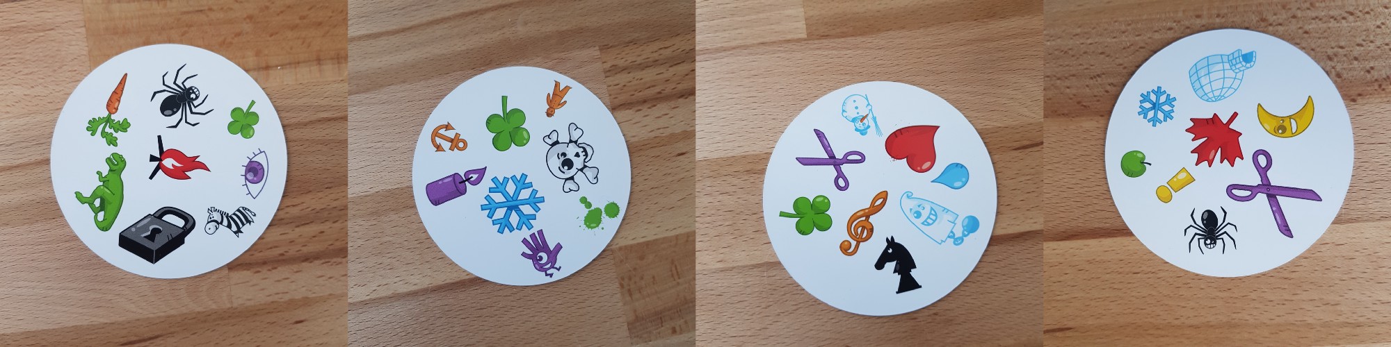
Image processing
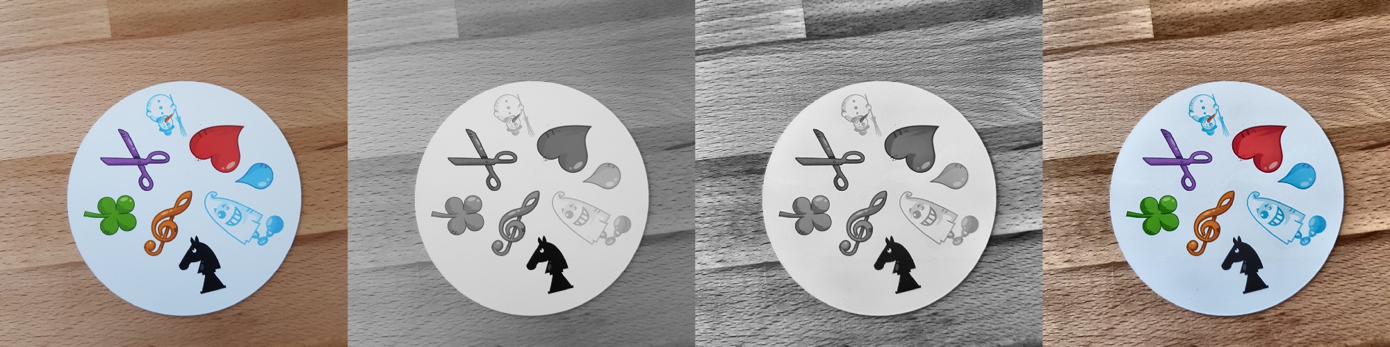
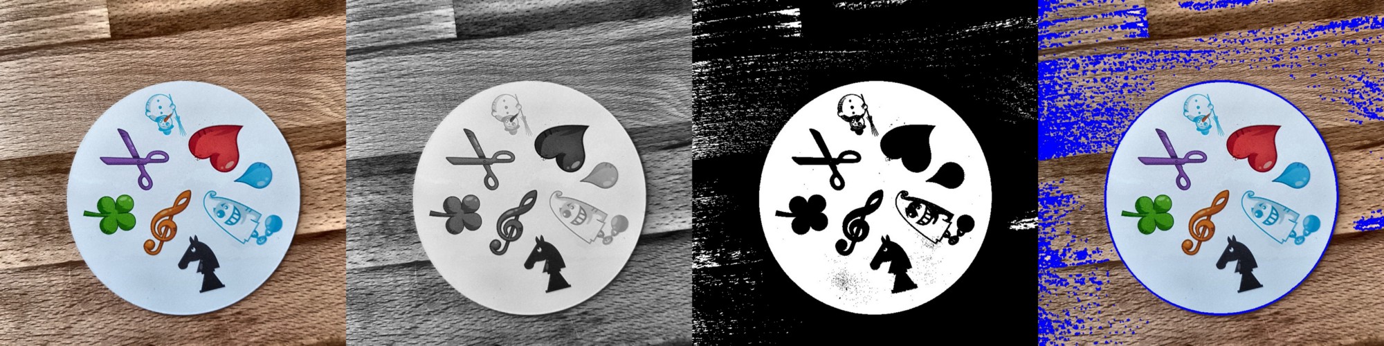
OK, the data we have, what's next? Probably the most important part on the path to success: image processing. We need to get characters from each image. Some difficulties await us here. In the photos above, it is noticeable that some characters are more difficult to distinguish than others: the snowman and the ghost (in the third photo) and the needle (in the fourth) of light colors, and the blots (in the second photo) and the exclamation mark (in the fourth photo) consist of several parts . To process light characters we will add contrast. After that we will resize and save the image.Add contrast
To add contrast, we use the Lab color space . L is lightness, a is the chromatic component in the range from green to magenta, and b is the chromatic component in the range from blue to yellow. We can easily extract these components using OpenCV :import cv2
import imutils
imgname = 'picture1'
image = cv2.imread(f’{imgname}.jpg’)
lab = cv2.cvtColor(image, cv2.COLOR_BGR2LAB)
l, a, b = cv2.split(lab)
 From left to right: the original image, the lightness component, component a and component bNow we add contrast to the lightness component, again combine all the components together and convert to a normal image:
clahe = cv2.createCLAHE(clipLimit=3.0, tileGridSize=(8,8))
cl = clahe.apply(l)
limg = cv2.merge((cl,a,b))
final = cv2.cvtColor(limg, cv2.COLOR_LAB2BGR)
 From left to right: the original image, the lightness component, the image with high contrast and the image converted back to RGB
Change of size
Now resize and save the image:resized = cv2.resize(final, (800, 800))
# save the image
cv2.imwrite(f'{imgname}processed.jpg', blurred)
Done!Card and character recognition
Now that the image is processed, we can detect a card in the image. Using OpenCV, we are looking for external contours. Then we convert the image into halftones, select the threshold value (in our case, 190) to create a black-and-white image and search for a path. The code:image = cv2.imread(f’{imgname}processed.jpg’)
gray = cv2.cvtColor(image, cv2.COLOR_RGB2GRAY)
thresh = cv2.threshold(gray, 190, 255, cv2.THRESH_BINARY)[1]
# find contours
cnts = cv2.findContours(thresh.copy(), cv2.RETR_EXTERNAL, cv2.CHAIN_APPROX_SIMPLE)
cnts = imutils.grab_contours(cnts)
output = image.copy()
# draw contours on image
for c in cnts:
cv2.drawContours(output, [c], -1, (255, 0, 0), 3)
 Processed image converted into halftones using threshold and selecting external contoursIf we sort the external contours by area, we will find the contour with the largest area - this will be our card. To extract the characters we can create a white background.
# sort by area, grab the biggest one
cnts = sorted(cnts, key=cv2.contourArea, reverse=True)[0]
# create mask with the biggest contour
mask = np.zeros(gray.shape,np.uint8)
mask = cv2.drawContours(mask, [cnts], -1, 255, cv2.FILLED)
# card in foreground
fg_masked = cv2.bitwise_and(image, image, mask=mask)
# white background (use inverted mask)
mask = cv2.bitwise_not(mask)
bk = np.full(image.shape, 255, dtype=np.uint8)
bk_masked = cv2.bitwise_and(bk, bk, mask=mask)
# combine back- and foreground
final = cv2.bitwise_or(fg_masked, bk_masked)
 Mask, background, foreground image, final imageNow it's time for character recognition! We can use the resulting image to detect external contours on it again, these contours will be symbols. If we create a square around each symbol, we can extract this area. Here the code is a little longer:
gray = cv2.cvtColor(final, cv2.COLOR_RGB2GRAY)
thresh = cv2.threshold(gray, 195, 255, cv2.THRESH_BINARY)[1]
thresh = cv2.bitwise_not(thresh)
cnts = cv2.findContours(thresh.copy(), cv2.RETR_EXTERNAL, cv2.CHAIN_APPROX_SIMPLE)
cnts = imutils.grab_contours(cnts)
cnts = sorted(cnts, key=cv2.contourArea, reverse=True)[:10]
i = 0
for c in cnts:
if cv2.contourArea(c) > 1000:
mask = np.zeros(gray.shape, np.uint8)
mask = cv2.drawContours(mask, [c], -1, 255, cv2.FILLED)
fg_masked = cv2.bitwise_and(image, image, mask=mask)
mask = cv2.bitwise_not(mask)
bk = np.full(image.shape, 255, dtype=np.uint8)
bk_masked = cv2.bitwise_and(bk, bk, mask=mask)
finalcont = cv2.bitwise_or(fg_masked, bk_masked)
output = finalcont.copy()
x,y,w,h = cv2.boundingRect(c)
if w < h:
x += int((w-h)/2)
w = h
else:
y += int((h-w)/2)
h = w
roi = finalcont[y:y+h, x:x+w]
roi = cv2.resize(roi, (400,400))
cv2.imwrite(f"{imgname}_icon{i}.jpg", roi)
i += 1
 Black and white image (thresholded), detected outlines, a ghost symbol and a heart symbol (characters extracted with masks)
Character sort
And now the most boring! You need to sort the characters. You will need the train, test, and validation directories, 57 directories each (we have 57 different characters in total). The folder structure is as follows:symbols
├── test
│ ├── anchor
│ ├── apple
│ │ ...
│ └── zebra
├── train
│ ├── anchor
│ ├── apple
│ │ ...
│ └── zebra
└── validation
├── anchor
├── apple
│ ...
└── zebra
It will take some time to put the extracted characters (more than 2500 pieces) in the necessary directories! I have code for creating subfolders, a test suite and a validation kit on GitHub . Maybe next time it’s better to do the sorting based on the clustering algorithm ...Convolutional neural network training
After the boring part, the fun comes again! It's time to create and train a convolutional neural network. You can find information about convolutional neural networks here .Model architecture
We have the task of multi-class classification with one label. For each character we need one label. That is why we will need a function to activate the output softmax layer with 57 nodes and categorical cross-entropy as a loss function.The architecture of the final model is as follows:
from keras import layers
from keras import models
from keras import optimizers
from keras.preprocessing.image import ImageDataGenerator
import matplotlib.pyplot as plt
model = models.Sequential()
model.add(layers.Conv2D(32, (3, 3), activation='relu', input_shape=(400, 400, 3)))
model.add(layers.MaxPooling2D((2, 2)))
model.add(layers.Conv2D(64, (3, 3), activation='relu'))
model.add(layers.MaxPooling2D((2, 2)))
model.add(layers.Conv2D(128, (3, 3), activation='relu'))
model.add(layers.MaxPooling2D((2, 2)))
model.add(layers.Conv2D(256, (3, 3), activation='relu'))
model.add(layers.MaxPooling2D((2, 2)))
model.add(layers.Conv2D(256, (3, 3), activation='relu'))
model.add(layers.MaxPooling2D((2, 2)))
model.add(layers.Conv2D(128, (3, 3), activation='relu'))
model.add(layers.Flatten())
model.add(layers.Dropout(0.5))
model.add(layers.Dense(512, activation='relu'))
model.add(layers.Dense(57, activation='softmax'))
model.compile(loss='categorical_crossentropy', optimizer=optimizers.RMSprop(lr=1e-4), metrics=['acc'])
Data Augmentation
To improve performance, I used data augmentation. Data augmentation is the process of increasing the volume and variety of input data. This can be done by rotating, shifting, scaling, cropping and flipping existing images. Keras can easily augment data:
train_dir = 'symbols/train'
validation_dir = 'symbols/validation'
test_dir = 'symbols/test'
train_datagen = ImageDataGenerator(rescale=1./255, rotation_range=40, width_shift_range=0.1, height_shift_range=0.1, shear_range=0.1, zoom_range=0.1, horizontal_flip=True, vertical_flip=True)
test_datagen = ImageDataGenerator(rescale=1./255)
train_generator = train_datagen.flow_from_directory(train_dir, target_size=(400,400), batch_size=20, class_mode='categorical')
validation_generator = test_datagen.flow_from_directory(validation_dir, target_size=(400,400), batch_size=20, class_mode='categorical')
If you were interested, the augmented ghost looks like this: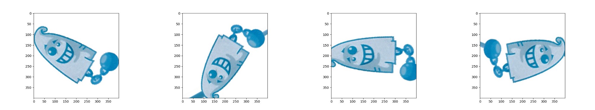 The original image of the ghost on the left, augmented ghosts in all the other pictures
Model training
Let's train the model, save it to use for predictions, and check the results.history = model.fit_generator(train_generator, steps_per_epoch=100, epochs=100, validation_data=validation_generator, validation_steps=50)
model.save('models/model.h5')
 Perfect predictions!
results
The basic model that I trained without data augmentation, dropouts and with fewer layers. This model gave the following results: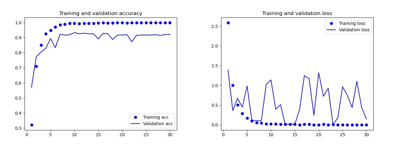 The results of the basic modelWith the naked eye, it is clear that this model is retrained. The results of the final version of the model (its code is presented in the previous sections) are much better. On the graph below you can see the accuracy and losses during training and on the validation set.
 Results of the final model.On the test set, this model made only one mistake, it recognized the bomb as a drop. I decided to stay on this model, the accuracy on the test set was 0.995.
Recognition of a common symbol on two cards
Now you can start looking for common symbols on two cards. We use two photographs, we will make predictions for each image separately and use the intersection of sets to find out which symbol is on both cards. We have 3 work options:- Something went wrong during the prediction: no common characters were found.
- There is one symbol at the intersection (prediction can be true or false).
- There is more than one character at the intersection. In this case, I choose the symbol with the highest probability (the average of both predictions).
The code for predicting all the combination on the two images in the catalog lies with GitHub 's main.py.And here are the results:
Conclusion
Isn't that the perfect model? Unfortunately no. When I took new photos of the cards and gave them the models for prediction, there were some problems with the snowman. Sometimes he recognized the eye or zebra as a snowman! As a result, sometimes the results were strange: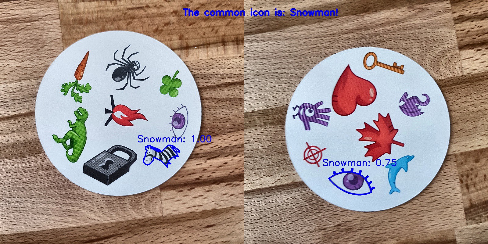 Well, where is the snowman here?Is this model better than man? Depending on what we need: people recognize perfectly, but the model does it faster! I noticed the time for which the computer is coping: I gave a deck of 55 cards and I had to get a common symbol for each combination of two cards. In total, these are 1485 combinations. The computer did it in less than 140 seconds. He made a few mistakes, but he will definitely beat any person when it comes to speed!
 I don’t think that creating a working 100% model is difficult. This can be achieved through transfer training. To understand what the model does, we could visualize layers for the test image. You can do it next time!
Learn more about the course and pass the entrance test