Python genetic algorithm for finding global extrema

Background

Recently, in the framework of educational activities, I needed to use the good old genetic algorithm in order to find the minimum and maximum functions of two variables. However, to my surprise, there was no similar implementation on python on the Internet, and this section was not covered in the article on the genetic algorithm on Wikipedia.



And so I decided to write my small package in Python with a visualization of the algorithm, according to which it will be convenient to configure this algorithm and look for the subtleties of the selected model.

In this short article, I would like to share the process, observations, and outcomes.

The principle of the algorithm

I will not talk about the global principle of the work of genetic algorithms, but if you have not heard about this, then you can familiarize yourself with it on Wikipedia .

At the moment, only one GA is implemented in the package, which is parameterized by the input data through a simple guic. I will tell you briefly about the selected genetic functions and basic algorithmic solutions.

The monochromosomal individual carries in each of its gene information about the corresponding x or y coordinate. A population is determined by many individuals, but the population is segmented into 4 individuals. This solution, of course, is due to an attempt to avoid convergence to a local optimum, since the task is to find a global extremum. Such a partition, as practice has shown, in many cases does not allow one genotype to dominate in the entire population, but, on the contrary, gives “evolution” greater dynamics. For each such part of the population, the following algorithm is applied:

1. Selection takes place similar to the ranking method. 3 individuals with the best fitness function indicators are selected (i.e., individuals are sorted in ascending / descending order of a function specified by the user, which acts as the adaptation function).
2. Next, the crossing function is applied in such a way that a new generation (or rather a new segment of a population of 4 individuals) receives 2 pairs of unmuted genes from an individual with a better indication of fitness function and a pair of mutated genes from two other individuals. More on the compilation of the mutation function will be written in the next section.

The principle of operation of selection, crossbreeding and mutation visually looks like this (in generation N, the chromosomes of individuals are already sorted in the right order, and a small black square means mutation):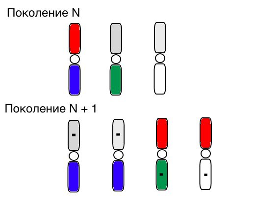

Primary tests and observations

So, we test this algorithm on two simple examples:

Test 1

$$

$$f(x, y) = sin(x) + cos(y)$$

Test 2

$$

$$\frac{4 \sqrt{x} - 5y }{ 3x ^ 2 + 2 y ^ 2 - 2 x + 1}$$

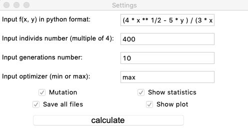
After testing and studying the operation of the algorithm by the method of gaze and random poking, several hypotheses-patterns were revealed:

• , ,

• $$

  $$[-1, 1)$$
  - . , , , ( )
• 5-15 , «»
• The zero generation is filled with random numbers only in a square

  $$

  $$[-1, 1)*[-1, 1)$$
  
  and there may be cases when this square covers a local extremum, which does not suit us

Consider a surface with many extrema of the form:

$$

$$g(x, y) = \sum\limits_{i=1}^nf_n(h, x_0, y_0), f(h, x_0, y_0) = h*exp(-(x - x_0)^2 - (y - y_0)^2)$$

The extrema of the function g will be at points

$$

$$(x_0, y_0)$$

.

Test 3

$$

$$g(x, y) = f_1(2, 0, 0) + f_2(5, 3, 3)$$

$$

$$g(x, y) = 2exp(-x^2 - y^2) + 5exp(-(x - 3)^2 - (y - 3)^2)$$

This example confirms and illustrates all the above observations.

Genetic Algorithm Upgrade

So, at the moment, the mutation function is composed very primitively: it adds random values ​​from the half-interval

$$

$$[-1, 1)$$

to the mutated gene. Such mutation invariance sometimes interferes with the correct operation of the algorithm, but there is an effective way to correct this defect.

We introduce a new parameter, which we will call the “mutation range” and which will show in which half-interval the gene mutates. Let us make this mutation coefficient inversely proportional to the generation number. Those. the higher the generation number, the weaker the genes mutate. This solution allows you to customize the start area and improve the accuracy of calculations if necessary.

Test 1

$$

$$f(x, y) = sinx$$

As the example shows, now, with each generation, the population converges more and more to the point of extremum and calculates the most accurate values ​​due to weak fluctuations.

But what about the problem of local extremes? Consider a familiar example.

Test 2

$$

$$g(x, y) = f_1(2, 0, 0) + f_2(5, 3, 3)$$

$$

$$g(x, y) = 2exp(-x^2 - y^2) + 5exp(-(x - 3)^2 - (y - 3)^2)$$

We see that now the idea of ​​dividing the population into parts works as intended. Without this segmentation, individuals of early generations could reveal a false dominant genotype at a local extremum, which would lead to an incorrect answer in the task. Also noticeable is a qualitative improvement in the accuracy of the answer due to the introduced dependence of the mutation on the generation number.

Summary

I summarize the result:

• The correct set of parameters allows you to accurately find the global extremum of a function of two variables
• ,
• ,

...

• , . , , aka
• , ,
• ()