Computer vision technology allows in today's realities to make life and business easier, cheaper, safer. According to various experts, this market will move in the coming years only in the direction of growth, which allows the development of appropriate technologies in the direction of productivity and quality. One of the most popular sections is Object Detection (object detection) - the definition of an object in the image or in the video stream.

The times when the detection of objects was solved exclusively through classical machine learning (cascades, SVM ...) have already passed - now approaches based on Deep Learning reign in this area. In 2014, an approach was proposed that significantly influenced subsequent research and development in this area - the R-CNN model. Its subsequent improvements (in the form of Fast R-CNN and Faster R-CNN) made it one of the most accurate, which has become the reason for its use to this day.

In addition to R-CNN, there are many more approaches that search for objects: the Yolo family, SSD, RetinaNet, CenterNet ... Some of them offer an alternative approach, while others are developing the current one in the direction of increasing the performance indicator. A discussion of almost each of them can be put out in a separate article, due to the abundance of chips and tricks :)

To study, I propose a set of articles with analysis of two-stage Object Detection models. The ability to understand their device brings an understanding of the basic ideas used in other implementations. In this post we will consider the most basic and, accordingly, the first of them - R-CNN.

Terminology

The bounding box — the coordinates that bound a specific area of ​​an image — most often in the shape of a rectangle. It can be represented by 4 coordinates in two formats: centered ($$$c_{x},c_{y},w,h$) and regular ($$$x_{min},y_{min},x_{max},y_{max}$)

Hypothesis (Proposal), P - a certain region of the image (specified using the bounding box) in which the object is supposedly located.

End-to-end training - training in which raw images arrive at the network input, and ready-made answers come out.

IoU (Intersection-over-Union) - metric of the degree of intersection between two bounding boxes.

R-CNN

One of the first approaches applicable for determining the location of an object in a picture is R-CNN (Region Convolution Neural Network). Its architecture consists of several successive steps and is illustrated in Figure 1:

1. Defining a set of hypotheses.
2. Extracting features from prospective regions using a convolutional neural network and encoding them into a vector.
3. The classification of an object within a hypothesis based on the vector from step 2.
4. Improvement (adjustment) of the coordinates of the hypothesis.
5. Everything repeats from step 2 until all hypotheses from step 1 are processed.

Consider each step in more detail.

Hypothesis Search

Having a specific image at the input, the first thing it breaks down into small hypotheses of different sizes. The authors of this article use Selective Search - top-level, it allows you to compile a set of hypotheses (the class of the object does not matter yet), based on segmentation to determine the boundaries of objects by pixel intensity, color difference, contrast and texture. At the same time, the authors note that any similar algorithm can be used. Thus, approximately 2,000 different regions stand out, which partially overlap each other. For more accurate subsequent processing, each hypothesis is further expanded by 16 pixels in all 4 directions - as if adding context .

Total:

• Input: original image.
• Output: a set of hypotheses of different sizes and aspect ratios.

Image encoding

Each hypothesis from the previous step independently and separately from each other enters the input of the convolutional neural network. As it uses the architecture of AlexNet without the last softmax-layer. The main task of the network is to encode the incoming image into a vector representation that is extracted from the last fully connected FC7 layer. So the output is a 4096-dimensional vector representation.

You can notice that the input of AlexNet has a dimension of 3 × 227 × 227, and the size of the hypothesis can be almost any aspect ratio and size. This problem is bypassed by simply compressing or stretching the input to the desired size.

Total:

• Input: each hypothesis proposed in the previous step.
• Output: vector representation for each hypothesis.

Classification

After obtaining the vector characterizing the hypothesis, its further processing becomes possible. To determine which object is located in the intended region, the authors use the classic SVM-based separation plane classification method (Support Vector Machine - a support vector machine, can be modeled using Hinge loss ). And it should be$$$N_{c}+1$ individual (here, $$$N_{c}$denotes the number of defined classes of objects, and a unit is added to separately determine the background) of models trained according to the OvR principle (One vs. Rest - one against all, one of the methods of multiclass classification). In fact, the binary classification problem is being solved - is there a concrete class of an object inside the proposed region or not. So the way out is$$$N_{c}+1$-dimensional vector representing confidence in a particular class of the object contained in the hypothesis (the background is historically denoted by the zero class,$$$C_{i}=0$)

Total:

• Input: the vector of each of the proposed hypotheses from the penultimate layer of the network (in the case of AlexNet, this is FC7).
• Output: after sequentially launching each hypothesis, we obtain a dimension matrix $$$2000×N_{c}$representing the class of the object for each hypothesis.

Specification of hypotheses coordinates

The hypotheses obtained in step 1 do not always contain the correct coordinates (for example, an object can be “cropped” unsuccessfully), so it makes sense to correct them additionally. According to the authors, this brings an additional 3-4% to the metrics. So, hypotheses containing an object (the presence of an object is determined at the classification step) are additionally processed by linear regression. That is, hypotheses with the “background” class do not need additional processing of regions, because in fact there is no object there ...

Each object, specific to its class, has certain sizes and aspect ratios, therefore, which is logical, it is recommended to use our own regressor for each class .

Unlike the previous step, the authors use a non-vector from the FC7 layer for input to work best, and feature maps extracted from the last MaxPooling layer (in AlexNet, $$$MaxPool_{5}$, dimension 256 × 6 × 6). The explanation is the following - the vector stores information about the presence of an object with some characteristic details, and the feature map best stores information about the location of objects.

Total:

• Input: a map of attributes from the last MaxPooling layer for each hypothesis that contains any object except the background.
• Output: corrections to the coordinates of the bounding box of the hypothesis.

Helper Tricks

Before proceeding to the details of model training, we will consider two necessary tricks that we will need later.

Designation of positive and negative hypotheses

When teaching with a teacher, a certain balance between classes is always necessary. The converse can lead to poor classification accuracy. For example, if in a sample with two classes the first occurs only in a few percent of cases, then it is difficult for the network to learn how to determine it, because it can be interpreted as an outlier. In the case of Object Detection tasks, there is just such a problem - in the picture with a single object, only a few hypotheses (from ~ 2000) contain this very object ($$$C_{i}>0$), and everyone else is the background ($$$C_{i}=0$)

We accept the necessary notation: hypotheses containing objects will be called positive (positive), and without objects (containing only the background, or an insignificant part of the object) - negative (negative).

In order to subsequently determine the intersection between the two regions of the image, the Intersection over Union metric will be used . It is considered quite simple: the intersection area of ​​two regions is divided by the total area of ​​the regions. In the image below you can see illustrations of examples of metric counting.



With positive hypotheses, everything is clear - if the class is defined incorrectly, you need to be fined. But what about the negative? There are many more than positive ones ... To begin with, we note that not all negative hypotheses are equally difficult to recognize. For example, cases containing only the background ( easy negative ) are much easier to classify than containing another object or a small part of the desired ( hard negative ).

In practice, easy negative and hard negative are determined by the intersection of the bounding box (just used Intersection over Union) with the correct position of the object in the image. For example, if there is no intersection, or it is extremely small, this is easy negative ($$$C_{i}=0$) if large is hard negative or positive.

The Hard Negative Mining approach suggests using only hard negative for training, because, having learned to recognize them, we automatically achieve the best work with easy negative hypotheses. But such an ideology will be applied only in subsequent implementations (starting with Fast R-CNN).

Non-maximum suppression

Quite often, it turns out that the model identifies several hypotheses with great confidence pointing to the same object. Using Non-maximum suppression (NMS), you can handle such cases and leave only one, best, bounding box. But at the same time, do not forget about the case when the image can have two different objects of the same class. Figure 3 illustrates the effect of the operation before (left) and after (right) the operation of the algorithm.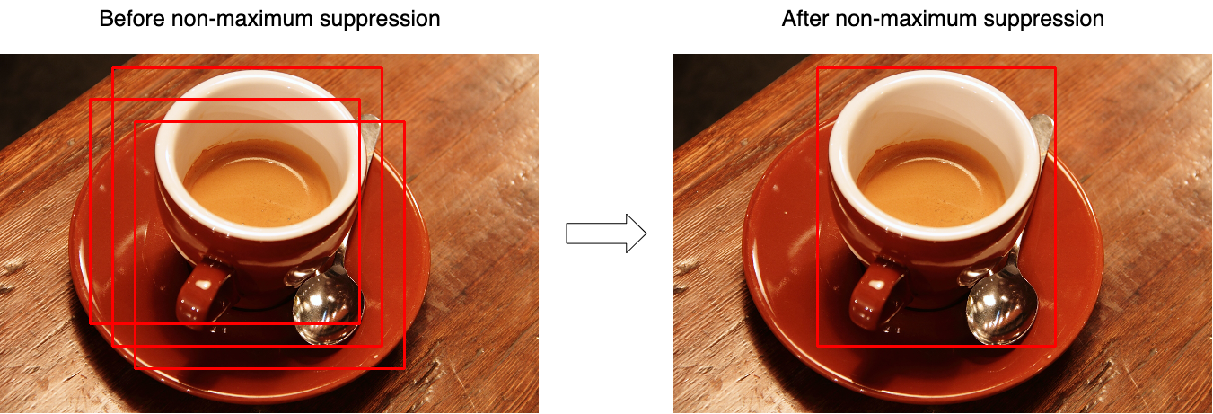



Consider the algorithm for working on one class (in reality, it is applied to each class separately):

1. At the input, the function takes a set of hypotheses for one class and a threshold that sets the maximum intersection between hypotheses.
2. Hypotheses are sorted by their "confidence."
3. In the cycle, the first hypothesis is selected (it has the highest confidence value) and is added to the result set.
4. In the cycle, the next, second hypothesis is selected (among those remaining after step 3).
5. If the intersection between the selected hypotheses is greater than the selected threshold (the intersection is calculated on the basis of the Intersection of Union), then the second hypothesis is discarded and is not further present in the result set.
6. Everything repeats from step 3 until the hypotheses are completely enumerated.

The pseudocode looks like this:

function nms(hypotheses, threshold):
    sorted = sort(hypotheses.values, key=hypotheses.scores)
    result = []
    for first in sorted:
        result.join(first)
        without_first = sorted / first
        for second in without_first:
            if IoU(first, second) > threshold:
                 sorted.remove(second)
    return result

Training

The hypothesis isolation block is not learningable.

Since the network is divided into several blocks that are separate from each other, it cannot be trained on an end-to-end basis. So, learning is a sequential process.

Vector View Training

The network pre-trained on ImageNet is taken as the basis - such networks already can well extract important features from incoming images, it remains to train them to work with the necessary classes. To do this, change the dimension of the output layer to$$$N_{c}$and train an already modified version. The first layers can be blocked, because they extract the primary (almost identical for all images) features, and the subsequent ones during training adapt to the features of the desired classes. So convergence will be achieved much faster. But if the training is still going badly, you can unlock the primary layers. Since it is necessary to precisely adjust the existing weights. It is not recommended to use a high learning rate (learning rate) - you can very quickly wipe existing weights.

When the network has learned to classify objects well, the last layer with SoftMax activation is discarded and the FC7 layer becomes the output, the output of which in turn can be interpreted as a vector representation of the hypothesis.

Positive at this step are hypotheses that intersect with the correct position of the object (IoU) by more than 0.5. All others are considered negative. To update the scales, a 128 mini-batch is used, consisting of 32 positive and 96 negative hypotheses.

Classifier Training

Let me remind you, to classify each hypothesis, $$$N_{c}+1$SVM models that receive the input of the vector representation of the hypothesis, and based on the principle of one against the other (One-vs-Rest) determine the class of the object. They are trained as ordinary SVM models with one exception - at this step the definition of positives and negatives is slightly different. Here the hypotheses are taken as negatives, the intersection of which with the correct position is less than 0.3.

Regress Training

Denote:

• $$$G=(g_{x},g_{y},g_{w},g_{h})$- the correct coordinates of the object;
• $$$\hat{G}=(\hat{g_{x}},\hat{g_{y}},\hat{g_{w}},\hat{g_{h}})$- corrected position of the hypotheses coordinates (must coincide with $$$G$);
• $$$T=(t_{x},t_{y},t_{w},t_{y})$- correct corrections to the coordinates;
• $$$P=(p_{x},p_{y},p_{w},p_{h})$- coordinates of the hypothesis;

So regressors (one for each class) represent four functions:

• $$$d_{x}(P)$, $$$d_{y}(P)$- determine the corrections to the center coordinates ($$$x,y$) To achieve the effect of independence from the original size, the correction should be normalized.
• $$$d_{w}(P)$and $$$d_{h}(P)$- determine the corrections to the width and height in the logarithmic space (the logarithmic space is used for numerical stability, and division - to determine the direction of the correction).

Denote by $$$\varphi_{5}(P)$feature map obtained from $$$MaxPool_{5}$network layer (recall, it has a dimension of 256 × 6 × 6, then it is simply stretched), when a hypothesis is limited to the coordinates by applying to the network $$$P$. We will look for a transformation$$$P$ at $$$G$like:

\ begin {align} Moreover $$\begin{align} \hat{g_x} &= p_w d_x(P) + p_x \\ \hat{g_y} &= p_h d_y(P) + p_y \\ \hat{g_w} &= p_w e^{d_w(P)} \\ \hat{g_h} &= p_h e^{d_h(P)} \end{align}$$
$$$d_{*}(P)={w_{*}}^{T}\varphi_{5}(P)$(here $$$*∈(x,y,w,h)$) is a linear function, and the vector $$$w_{*}$is searched using the optimization problem (ridge regression):

$$

$$w_{*}=argmax_{\hat{w_{*}}}\sum_{i}^{N}(T_{i_{*}}-d_{*}(P))^{2}+\lambda \left \| \hat{w_{x}} \right \|^{2}$$

To determine the corrections to the coordinates, we collect pairs between the correct position of the hypotheses $$$G$and their current state $$$P$, and define the values $$$T_{*}$like:

\ begin {align} The notation in the formulas inside this article may differ from the notation of the original article for the best understanding. Since there are ~ 2000 hypotheses on the output of the network, they are combined using Non-maximum suppression. The authors of the article also indicate that if instead of SVM you use the SoftMax layer (which was folded out in the second step), then the accuracy drops by ~ 4-4.5% (VOC 2007 dataset), but they note that the best “fit” of the scales will probably help to get rid from such a problem. $$\begin{align} T_x &= \frac{g_x-p_x}{p_w} \\ T_y &= \frac{g_y-p_y}{p_h} \\ T_w &= \log{\frac{g_w}{p_w}} \\ T_h &= \log{\frac{g_h}{p_h}}\qquad \end{align}$$

In conclusion, we highlight the main disadvantages of this approach:

1. The hypotheses proposed in step 1 can partially duplicate each other - different hypotheses can consist of identical parts, and each such hypothesis was separately processed by a neural network. It turns out that most network launches more or less duplicate each other unnecessarily.
2. It cannot be used for real-time operation, since ~ 53 seconds are spent on passing 1 image (frame) (NVIDIA Titan Black GPU).
3. The hypothesis extraction algorithm is not taught in any way, and therefore further improvement in quality is almost impossible (no one has canceled bad hypotheses).

This parses the very first R-CNN model. More advanced implementations (in the form of Fast R-CNN and Faster R-CNN) are discussed in a separate article .

Bibliography

1. R. Girshick, J. Donahue, T. Darrell, and J. Malik. “Rich feature hierarchies for accurate object detection and semantic segmentation.” In CVPR, 2014. arXiv: 1311.2524

2. R. Girshick, J. Donahue, T. Darrell, and J. Malik. “Region-based convolutional networks for accurate object detection and segmentation.” TPAMI, 2015

Posted by: Sergey Mikhaylin, Machine Learning Specialist, Jet Infosystems