Any activity generates data. Whatever you do, you probably have in your hands a storehouse of raw useful information, or at least access to its source.
Today the winner is the one who makes decisions based on objective data. The skills of the analyst are more relevant than ever, and the availability of the necessary tools at hand allows you to always be one step ahead. This is a help in the appearance of this article.
Do you have your own business? Or maybe ... though, it doesn't matter. The process of data mining is endless and exciting. And even just digging well on the Internet, you can find a field for activity.
Here's what we have today - An unofficial XML distribution database for RuTracker.ORG. The database is updated every six months and contains information on all distributions for the history of the existence of this torrent tracker.
What can she tell the owners of the rutracker? And the direct accomplices of piracy on the Internet? Or an ordinary user who is fond of anime, for example?
Do you understand what I mean?
Stack - R, Clickhouse, Dataiku
Any analytics goes through several main stages: data extraction, its preparation and data study (visualization). Each stage has its own tool. Because today's stack:
- R. , Python. dplyr ggplot2. – .
- Clickhouse. . : “clickhouse ” “ ”. , . .
- Dataiku. , -.
: Dataiku . 3 . .
, , , . dataiku .
Big Data – big problems
xml– 5 . – rutracker.org, (2005 .) 2019 . 15 !
R Studio – ! . , .
, R. Big Data, Clickhouse … , xml–. . .
. Dataiku DSS . – 10 000 . . , . , 200 000 .
, . .

. : content — json.
content, . – .
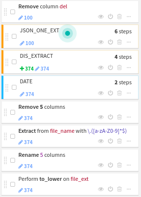
recipe — . , . json .
. , , + dataiku.
recipe, — .
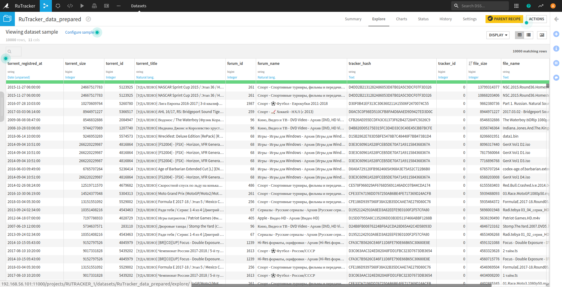
csv Clickhouse.
Clickhouse 15 rutracker-a.
?
SELECT ROUND(uniq(torrent_id) / 1000000, 2) AS Count_M
FROM rutracker

┌─Count_M─┐
│    1.46 │
└─────────┘
1 rows in set. Elapsed: 0.247 sec. Processed 25.51 million rows, 204.06 MB (103.47 million rows/s., 827.77 MB/s.)
1.5 25 . 0.3 ! .
, , .
SELECT COUNT(*) AS Count
FROM rutracker
WHERE (file_ext = 'epub') OR (file_ext = 'fb2') OR (file_ext = 'mobi')

┌──Count─┐
│ 333654 │
└────────┘
1 rows in set. Elapsed: 0.435 sec. Processed 25.51 million rows, 308.79 MB (58.64 million rows/s., 709.86 MB/s.)
300 — ! , . .
SELECT ROUND(SUM(file_size) / 1000000000, 2) AS Total_size_GB
FROM rutracker
WHERE (file_ext = 'epub') OR (file_ext = 'fb2') OR (file_ext = 'mobi')

┌─Total_size_GB─┐
│        625.75 │
└───────────────┘
1 rows in set. Elapsed: 0.296 sec. Processed 25.51 million rows, 344.32 MB (86.24 million rows/s., 1.16 GB/s.)
– 25 . , ?
R
R. , DBI ( ). Clickhouse.
Rlibrary(DBI) # , ... Clickhouse
library(dplyr) # %>%
#
library(ggplot2)
library(ggrepel)
library(cowplot)
library(scales)
library(ggrepel)
# localhost:9000
connection <- dbConnect(RClickhouse::clickhouse(), host="localhost", port = 9000)
, . dplyr .
? rutracker.org .
Ryears_stat <- dbGetQuery(connection,
"SELECT
round(COUNT(*)/1000000, 2) AS Files,
round(uniq(torrent_id)/1000, 2) AS Torrents,
toYear(torrent_registred_at) AS Year
FROM rutracker
GROUP BY Year")
ggplot(years_stat, aes(as.factor(Year), as.double(Files))) +
geom_bar(stat = 'identity', fill = "darkblue", alpha = 0.8)+
theme_minimal() +
labs(title = " RuTracker", subtitle = " 2005 - 2019\n")+
theme(axis.text.x = element_text(angle=90, vjust = 0.5),
axis.text.y = element_text(),
axis.title.y = element_blank(),
axis.title.x = element_blank(),
panel.grid.major.x = element_blank(),
panel.grid.major.y = element_line(size = 0.9),
panel.grid.minor.y = element_line(size = 0.4),
plot.title = element_text(vjust = 3, hjust = 0, family = "sans", size = 16, color = "#101010", face = "bold"),
plot.caption = element_text(vjust = 3, hjust = 0, family = "sans", size = 12, color = "#101010", face = "bold"),
plot.margin = unit(c(1,0.5,1,0.5), "cm"))+
scale_y_continuous(labels = number_format(accuracy = 1, suffix = " "))
ggplot(years_stat, aes(as.factor(Year), as.integer(Torrents))) +
geom_bar(stat = 'identity', fill = "#008b8b", alpha = 0.8)+
theme_minimal() +
labs(title = " RuTracker", subtitle = " 2005 - 2019\n", caption = "* ")+
theme(axis.text.x = element_text(angle=90, vjust = 0.5),
axis.text.y = element_text(),
axis.title.y = element_blank(),
axis.title.x = element_blank(),
panel.grid.major.x = element_blank(),
panel.grid.major.y = element_line(size = 0.9),
panel.grid.minor.y = element_line(size = 0.4),
plot.title = element_text(vjust = 3, hjust = 0, family = "sans", size = 16, color = "#101010", face = "bold"),
plot.caption = element_text(vjust = -3, hjust = 1, family = "sans", size = 9, color = "grey60", face = "plain"),
plot.margin = unit(c(1,0.5,1,0.5), "cm")) +
scale_y_continuous(labels = number_format(accuracy = 1, suffix = " "))
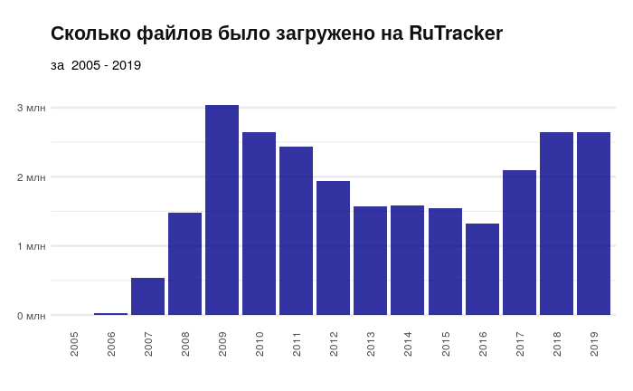
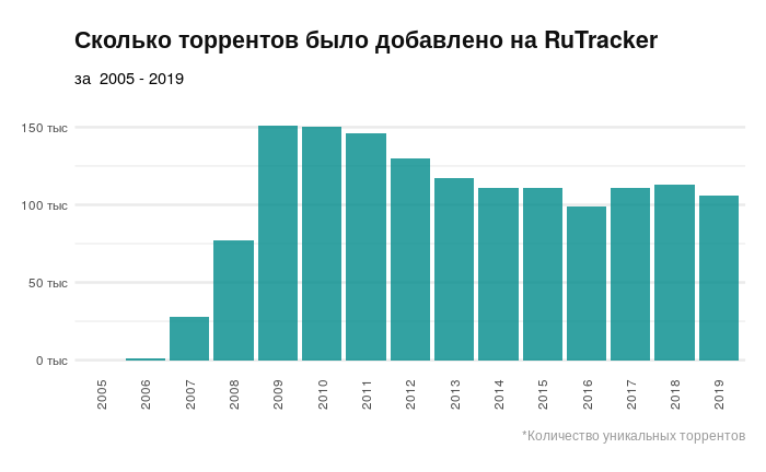
2016 . , 2016 rutracker.org . , .
, . , .
.
Rextention_stat <- dbGetQuery(connection,
"SELECT toYear(torrent_registred_at) AS Year,
COUNT(tracker_id)/1000 AS Count,
ROUND(SUM(file_size)/1000000000000, 2) AS Total_Size_TB,
file_ext
FROM rutracker
GROUP BY Year, file_ext
ORDER BY Year, Count")
#
TopExt <- function(x, n) {
res_tab <- NULL
# 2005 2006, ..
for (i in (3:15)) {
res_tab <-bind_rows(list(res_tab,
extention_stat %>% filter(Year == x[i]) %>%
arrange(desc(Count), desc(Total_Size_TB)) %>%
head(n)
))
}
return(res_tab)
}
years_list <- unique(extention_stat$Year)
ext_data <- TopExt(years_list, 5)
ggplot(ext_data, aes(as.factor(Year), as.integer(Count), fill = file_ext)) +
geom_bar(stat = "identity",position="dodge2", alpha =0.8, width = 1)+
theme_minimal() +
labs(title = " RuTracker",
subtitle = " 2005 - 2019\n",
caption = "* -5 ", fill = "") +
theme(axis.text.x = element_text(angle=90, vjust = 0.5),
axis.text.y = element_text(),
axis.title.y = element_blank(),
axis.title.x = element_blank(),
panel.grid.major.x = element_blank(),
panel.grid.major.y = element_line(size = 0.9),
panel.grid.minor.y = element_line(size = 0.4),
legend.title = element_text(vjust = 1, hjust = -1, family = "sans", size = 9, color = "#101010", face = "plain"),
legend.position = "top",
plot.title = element_text(vjust = 3, hjust = 0, family = "sans", size = 16, color = "#101010", face = "bold"),
plot.caption = element_text(vjust = -4, hjust = 1, family = "sans", size = 9, color = "grey60", face = "plain"),
plot.margin = unit(c(1,0.5,1,0.5), "cm")) +
scale_y_continuous(labels = number_format(accuracy = 0.5, scale = (1/1000), suffix = " "))+guides(fill=guide_legend(nrow=1))
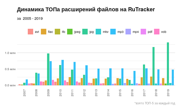
. . .
rutracker-a. .
Rchapter_stat <- dbGetQuery(connection,
"SELECT
substring(forum_name, 1, position(forum_name, ' -')) Chapter,
uniq(torrent_id) AS Count,
ROUND(median(file_size)/1000000, 2) AS Median_Size_MB,
ROUND(max(file_size)/1000000000) AS Max_Size_GB,
ROUND(SUM(file_size)/1000000000000) AS Total_Size_TB
FROM rutracker WHERE Chapter NOT LIKE('\"%')
GROUP BY Chapter
ORDER BY Count DESC")
chapter_stat$Count <- as.integer(chapter_stat$Count)
#
AggChapter2 <- function(Chapter){
var_ch <- str(Chapter)
res = NULL
for(i in (1:22)){
select_str <-paste0(
"SELECT
toYear(torrent_registred_at) AS Year,
substring(forum_name, 1, position(forum_name, ' -')) Chapter,
uniq(torrent_id)/1000 AS Count,
ROUND(median(file_size)/1000000, 2) AS Median_Size_MB,
ROUND(max(file_size)/1000000000,2) AS Max_Size_GB,
ROUND(SUM(file_size)/1000000000000,2) AS Total_Size_TB
FROM rutracker
WHERE Chapter LIKE('", Chapter[i], "%')
GROUP BY Year, Chapter
ORDER BY Year")
res <-bind_rows(list(res, dbGetQuery(connection, select_str)))
}
return(res)
}
chapters_data <- AggChapter2(chapter_stat$Chapter)
chapters_data$Chapter <- as.factor(chapters_data$Chapter)
chapters_data$Count <- as.numeric(chapters_data$Count)
chapters_data %>% group_by(Chapter)%>%
ggplot(mapping = aes(x = reorder(Chapter, Total_Size_TB), y = Total_Size_TB))+
geom_bar(stat = "identity", fill="darkblue", alpha =0.8)+
theme(panel.grid.major.x = element_line(colour="grey60", linetype="dashed"))+
xlab('\n') + theme_minimal() +
labs(title = "C RuTracker-",
subtitle = " 2019\n")+
theme(axis.text.x = element_text(),
axis.text.y = element_text(family = "sans", size = 9, color = "#101010", hjust = 1, vjust = 0.5),
axis.title.y = element_text(vjust = 2.5, hjust = 0, family = "sans", size = 9, color = "grey40", face = "plain"),
axis.title.x = element_blank(),
axis.line.x = element_line(color = "grey60", size = 0.1, linetype = "solid"),
panel.grid.major.y = element_blank(),
panel.grid.major.x = element_line(size = 0.7, linetype = "solid"),
panel.grid.minor.x = element_line(size = 0.4, linetype = "solid"),
plot.title = element_text(vjust = 3, hjust = 1, family = "sans", size = 16, color = "#101010", face = "bold"),
plot.subtitle = element_text(vjust = 2, hjust = 1, family = "sans", size = 12, color = "#101010", face = "plain"),
plot.caption = element_text(vjust = -3, hjust = 1, family = "sans", size = 9, color = "grey60", face = "plain"),
plot.margin = unit(c(1,0.5,1,0.5), "cm"))+
scale_y_continuous(labels = number_format(accuracy = 1, suffix = " "))+
coord_flip()
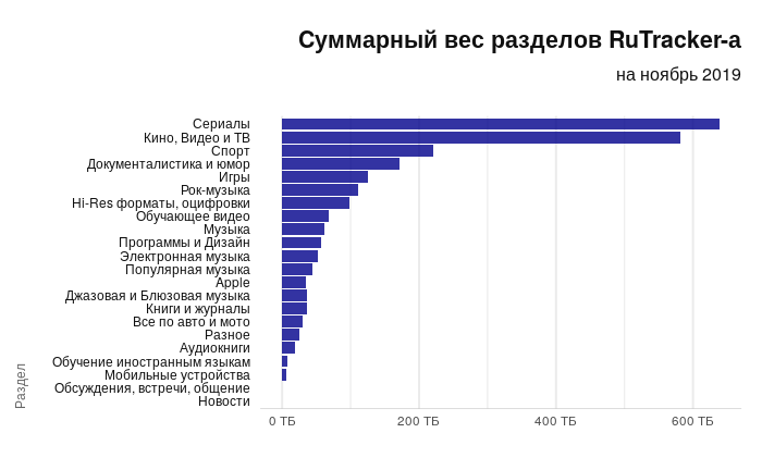
. — — . , . , Apple.
Rchapters_data %>% group_by(Chapter)%>%
ggplot(mapping = aes(x = reorder(Chapter, Count), y = Count))+
geom_bar(stat = "identity", fill="#008b8b", alpha =0.8)+
theme(panel.grid.major.x = element_line(colour="grey60", linetype="dashed"))+
xlab('') + theme_minimal() +
labs(title = " RuTracker-",
subtitle = " 2019\n")+
theme(axis.text.x = element_text(),
axis.text.y = element_text(family = "sans", size = 9, color = "#101010", hjust = 1, vjust = 0.5),
axis.title.y = element_text(vjust = 3.5, hjust = 0, family = "sans", size = 9, color = "grey40", face = "plain"),
axis.title.x = element_blank(),
axis.line.x = element_line(color = "grey60", size = 0.1, linetype = "solid"),
panel.grid.major.y = element_blank(),
panel.grid.major.x = element_line(size = 0.7, linetype = "solid"),
panel.grid.minor.x = element_line(size = 0.4, linetype = "solid"),
plot.title = element_text(vjust = 3, hjust = 1, family = "sans", size = 16, color = "#101010", face = "bold"),
plot.subtitle = element_text(vjust = 2, hjust = 1, family = "sans", size = 12, color = "#101010", face = "plain"),
plot.caption = element_text(vjust = -3, hjust = 1, family = "sans", size = 9, color = "grey60", face = "plain"),
plot.margin = unit(c(1,0.5,1,0.5), "cm"))+
scale_y_continuous(limits = c(0, 300), labels = number_format(accuracy = 1, suffix = " "))+
coord_flip()
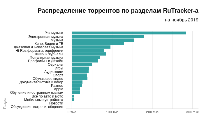
, , : -.
~15 .
Rlibrary("RColorBrewer")
getPalette = colorRampPalette(brewer.pal(19, "Spectral"))
chapters_data %>% #filter(Chapter %in% chapter_stat$Chapter[c(4,6,7,9:20)])%>%
filter(!Chapter %in% chapter_stat$Chapter[c(16, 21, 22)])%>%
filter(Year>=2007)%>%
ggplot(mapping = aes(x = Year, y = Count, fill = as.factor(Chapter)))+
geom_area(alpha =0.8, position = "fill")+
theme_minimal() +
labs(title = " -",
subtitle = " ~15 ", fill = "")+
theme(axis.text.x = element_text(vjust = 0.5),
axis.text.y = element_blank(),
axis.title.y = element_blank(),
axis.title.x = element_blank(),
panel.grid.major.x = element_blank(),
panel.grid.major.y = element_line(size = 0.9),
panel.grid.minor.y = element_line(size = 0.4),
plot.title = element_text(vjust = 3, hjust = 0, family = "sans", size = 16, color = "#101010", face = "bold"),
plot.caption = element_text(vjust = -3, hjust = 1, family = "sans", size = 9, color = "grey60", face = "plain"),
plot.margin = unit(c(1,1,1,1), "cm")) +
scale_x_continuous(breaks = c(2008, 2010, 2012, 2014, 2016, 2018),expand=c(0,0)) +
scale_fill_manual(values = getPalette(19))
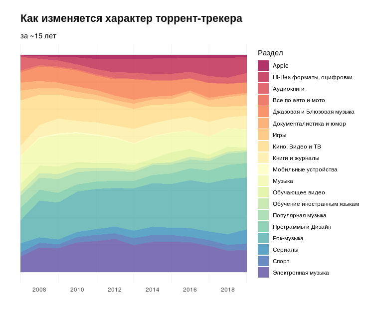
- — . — Apple , .
. .
, Rutracker-a. - rutracker.org.
Runique_torr_per_day <- dbGetQuery(connection,
"SELECT toDate(torrent_registred_at) AS date,
uniq(torrent_id) AS count
FROM rutracker
GROUP BY date
ORDER BY date")
unique_torr_per_day %>%
ggplot(aes(format(date, "%Y"), format(date, "%j"), fill = as.numeric(count)))+
geom_tile() +
theme_minimal() +
labs(title = " RuTracker-a",
subtitle = " ~15 \n\n",
fill = "- \n")+
theme(axis.text.x = element_text(vjust = 0.5),
axis.text.y = element_text(),
axis.title.y = element_blank(),
axis.title.x = element_blank(),
panel.grid.major.y = element_blank(),
panel.grid.major.x = element_line(size = 0.9),
panel.grid.minor.x = element_line(size = 0.4),
legend.title = element_text(vjust = 0.7, hjust = -1, family = "sans", size = 10, color = "#101010", face = "plain"),
legend.position = c(0.88, 1.30),
legend.direction = "horizontal",
plot.title = element_text(vjust = 3, hjust = 0, family = "sans", size = 16, color = "#101010", face = "bold"),
plot.caption = element_text(vjust = -3, hjust = 1, family = "sans", size = 9, color = "grey60", face = "plain"),
plot.margin = unit(c(1,1,1,1), "cm"))+ coord_flip(clip = "off") +
scale_y_discrete(breaks = c(format(as.Date("2007-01-15"), "%j"),
format(as.Date("2007-02-15"), "%j"),
format(as.Date("2007-03-15"), "%j"),
format(as.Date("2007-04-15"), "%j"),
format(as.Date("2007-05-15"), "%j"),
format(as.Date("2007-06-15"), "%j"),
format(as.Date("2007-07-15"), "%j"),
format(as.Date("2007-08-15"), "%j"),
format(as.Date("2007-09-15"), "%j"),
format(as.Date("2007-10-15"), "%j"),
format(as.Date("2007-11-15"), "%j"),
format(as.Date("2007-12-15"), "%j")),
labels = c("", "", "", "", "", "","", "", "", "","",""), position = 'right') +
scale_fill_gradientn(colours = c("#155220", "#c6e48b")) +
annotate(geom = "curve", x = 16.5, y = 119, xend = 13, yend = 135,
curvature = .3, color = "grey15", arrow = arrow(length = unit(2, "mm"))) +
annotate(geom = "text", x = 16, y = 45,
label = " « » \n",
hjust = "left", vjust = -0.75, color = "grey25") +
guides(x.sec = guide_axis_label_trans(~.x)) +
annotate("rect", xmin = 11.5, xmax = 12.5, ymin = 1, ymax = 366,
alpha = .0, colour = "white", size = 0.1) +
geom_segment(aes(x = 11.5, y = 25, xend = 12.5, yend = 25, colour = "segment"),
show.legend = FALSE)
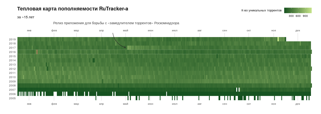
2017 . (. GitHub ). 2016 , . .
. . – .
, content , , , 15 .
Dataiku
, : , , , .
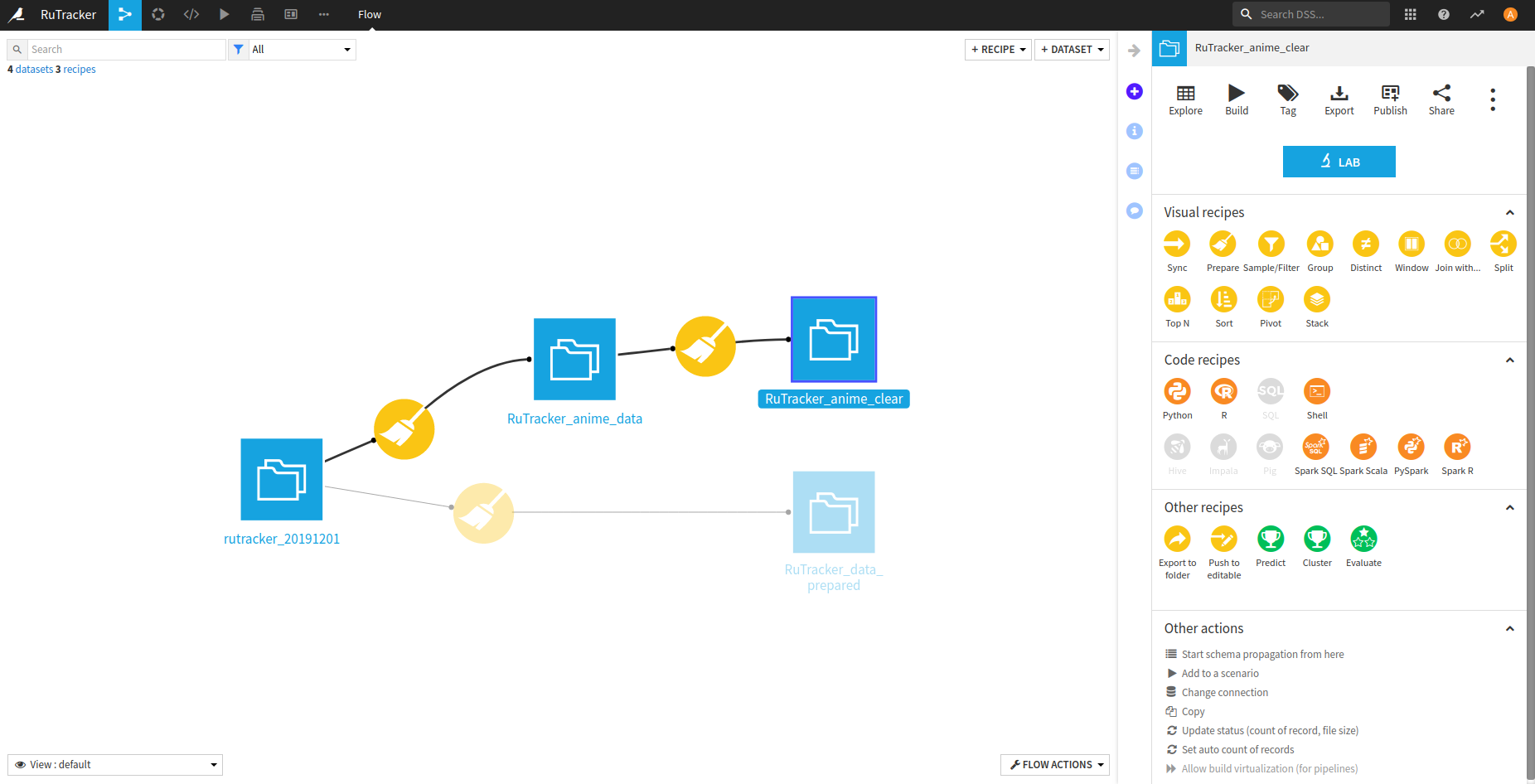
, -. . – .
– .
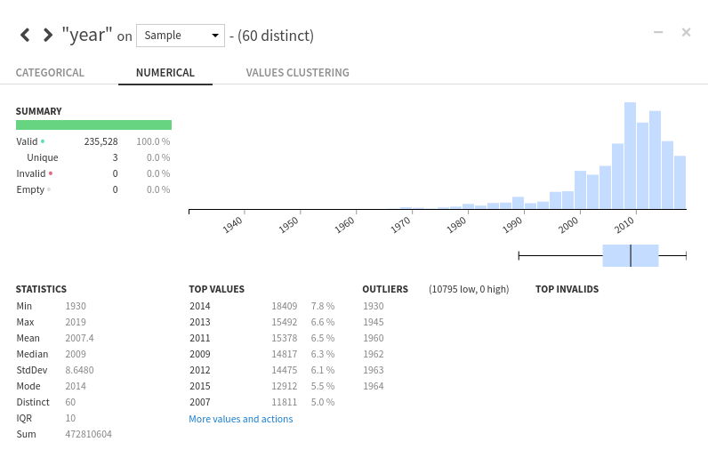
: rutracker.org , , — 60. 2009 — 2014 .
. , , . .
, . .

, dataiku — . , , (R, Python), . .
, RuTracker, : , . . , . .
UPD: , recipe dataiku.
Conditionally, the recipe given in this article can be divided into two parts: preparing data for analysis in R and preparing data about anime for analysis directly on the platform.
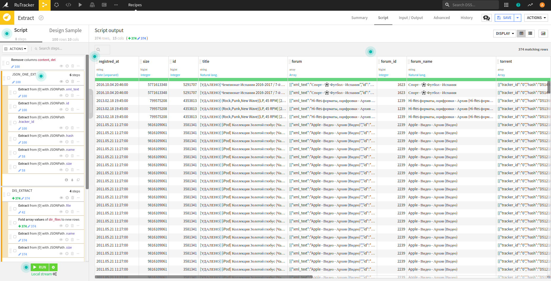
Stage of preparation for analysis in Rjson- .
json-. .
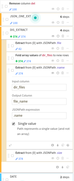
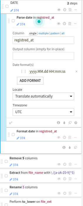
timestamp .
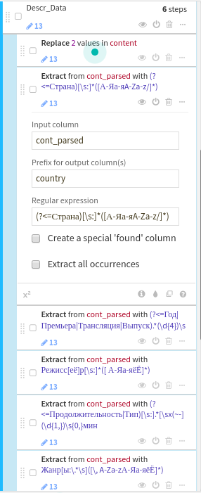
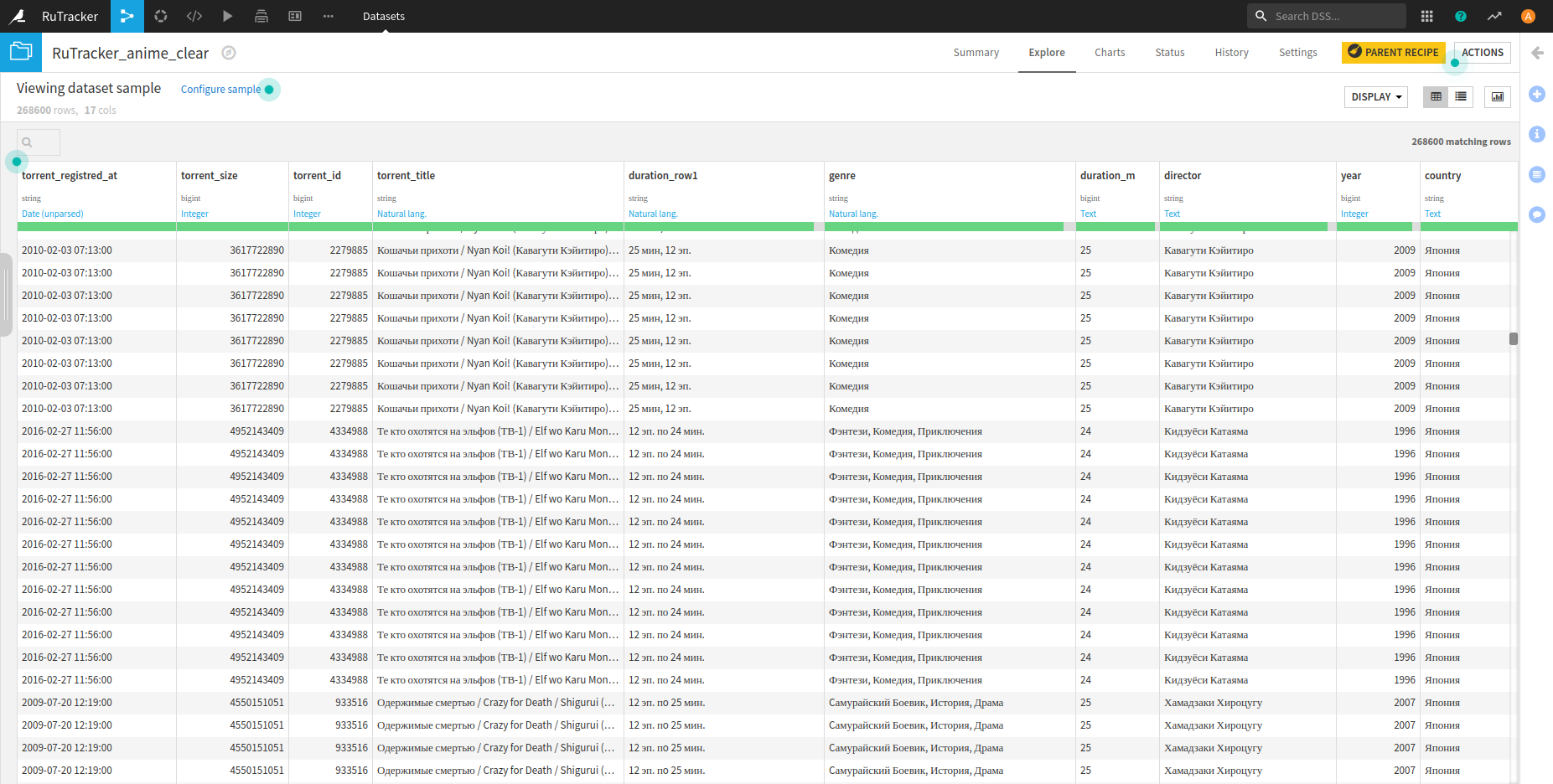
Stage of preparing anime data, , . content — Descr_Data.
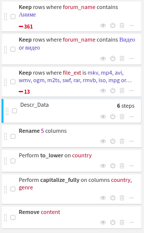
contentregexp , , , . , regexp dataiku .