There are a huge number of ways in which a robot can receive information from the outside world in order to interact with it. Also, depending on the tasks assigned to him, the methods of processing this information differ. In this article I will describe the main stages of the work carried out as part of the school project, the purpose of which is to systematize information on various methods of autonomous robot navigation and apply the knowledge gained in the process of creating the robot for the “RTK Cup” competitions.
Introduction
At the competitions “RTK Cup” there is a block of tasks that must be completed without operator intervention. I believe that many participants are unfairly avoiding these tasks, because the seemingly complexity of creating a robot design and writing a program hides largely simplified tasks from other competitive disciplines, combined in one training ground. By my project I want to show possible solutions to such problems, considering as an example the following along the line.To achieve the project goal, the following intermediate tasks were formulated:- Analysis of the rules of the competition “RTK Cup”
- Analysis of existing algorithms for autonomous orientation of a mobile robot
- Software creation
Analysis of the rules of the competition “RTK Cup”
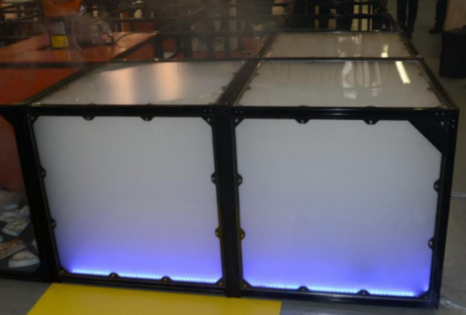
At the “RTK Cup” competitions, participants are presented with a training ground on which sections of varying complexity are modeled. The competition aims to stimulate young robotics to create devices that can work in extreme conditions, overcome obstacles, under human control, or autonomously.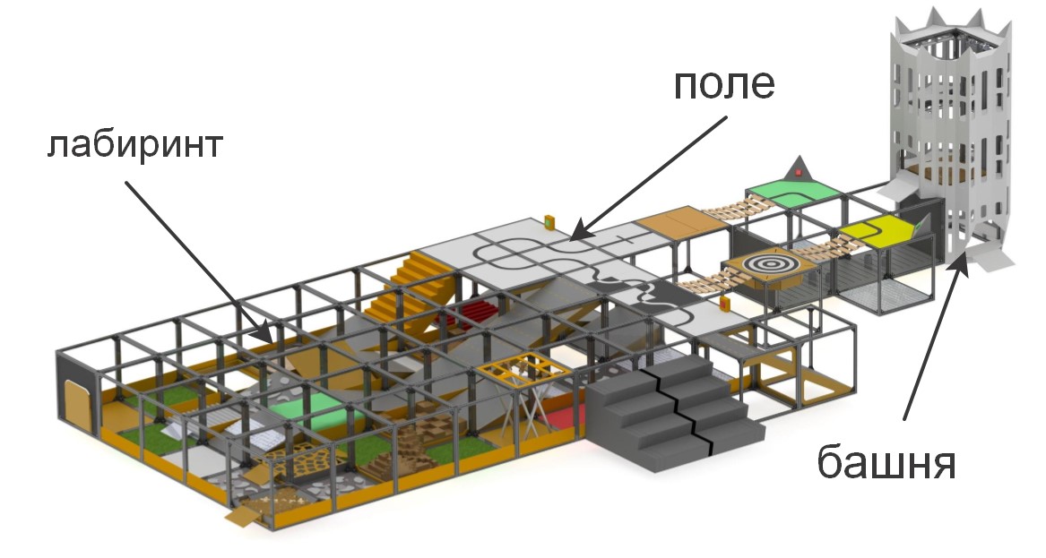
briefly about the elements that make up the polygon«» , . , , (), , (), ..
:
:

– , «» ( ) , . , , , , .
. , , , , , , .
Competitions are divided into two fundamentally different from each other nominations: “Seeker” and “Extreme”. This is to ensure that the competition was held between participants with a minimum difference in age and experience in developing robotic systems: Seeker for the younger level, and Extreme for participants from 14 years of age and older. In the Seeker nomination, the operator can freely move around the range and have direct eye contact with the machine, while the Extreme nomination assumes that the robot has video communication systems and / or computer vision, since the operator must navigate in the maze, relying only on the maze the camera and sensors built into the robot, while being behind a special screen.To qualify in competitions, the robot must either pass the task for remote control of the manipulator, or perform one of the elements of autonomy. In the framework of the project, the task was set to fulfill autonomy tasks, as they give the most points at the lowest cost from the operator. The elements of autonomy include:- Driving along a line with an ambient light sensor or a line of sight system
- Standalone beacon capture using distance sensor or vision systems
- Movement along a complex trajectory (for example, ascent / descent of stairs) along a line using a compass, gyroscope, accelerometer, vision system, or combined methods
Also, points for overcoming obstacles are doubled if the robot passes them autonomously.Within the framework of this project, the solution to the first of the tasks will be considered - movement along the line. The most common methods used when moving along the line are light sensors and a camera. The pluses of the sensors include the simplicity of creating a program - many of them are equipped with a tuning resistor, so that by setting the sensor for background lighting, it will give out 0 or 1, depending on whether it is on the line or not. For the same reason, light sensors are not demanding on the processing power of the controller used. Also, because of this, solving the problem with the help of light sensors is the least costly - the cost of the simplest sensor is 35 rubles, and for a relatively stable ride along the line, three sensors are enough (one is installed on the line, and two on the sides). However,One of the main disadvantages of such sensors is installation restrictions. Ideally, the sensor should be installed exactly in the center, at a small distance from the floor, otherwise it will give incorrect values. This is not a problem in specialized competitions where the robot must drive as fast as possible along the track, but, in the conditions of the “RTK Cup” competition, all of the above-mentioned sensor flaws can be critical - their installation primarily requires the presence of additional mechanical parts on the robot that raise and lowering the sensors, and this requires additional space on the robot, a separate engine moving the sensors, and is also a place of potential damage and increases the mass of the robot.otherwise it will give incorrect values. This is not a problem in specialized competitions where the robot must drive as fast as possible along the track, but, in the conditions of the “RTK Cup” competition, all of the above-mentioned sensor flaws can be critical - their installation primarily requires the presence of additional mechanical parts on the robot that raise and lowering the sensors, and this requires additional space on the robot, a separate engine moving the sensors, and is also a place of potential damage and increases the mass of the robot.otherwise it will give incorrect values. This is not a problem in specialized competitions where the robot must drive as fast as possible along the track, but, in the conditions of the “RTK Cup” competition, all of the above-mentioned sensor flaws can be critical - their installation primarily requires the presence of additional mechanical parts on the robot that raise and lowering the sensors, and this requires additional space on the robot, a separate engine moving the sensors, and is also a place of potential damage and increases the mass of the robot.all the above-mentioned sensor flaws can be critical - their installation primarily requires the presence of additional mechanical parts on the robot that raise and lower the sensors, and this requires additional space on the robot, a separate motor that moves the sensors, and is also a place of potential damage and increases the mass of the robot .all the above-mentioned sensor flaws can be critical - their installation primarily requires the presence of additional mechanical parts on the robot that raise and lower the sensors, and this requires additional space on the robot, a separate motor that moves the sensors, and is also a place of potential damage and increases the mass of the robot .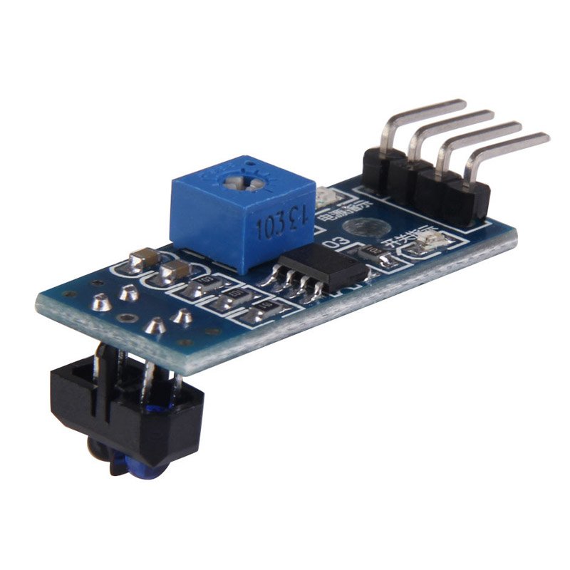 The camera, in turn, has the following advantages: it has a practically unlimited (in comparison with sensors) measurement radius, i.e. only one camera module is able to simultaneously see the line, both directly below the robot, and at a sufficient distance from it, which allows, for example, to evaluate its curvature and select a proportional control action. At the same time, the camera module does not interfere with the advancement of the robot in other parts of the landfill that do not require autonomy, since the camera is fixed at a distance from the floor. The main minus of the camera is that video processing requires a powerful computing complex on board the robot, and the software being developed needs more fine-tuning, because the camera receives an order of magnitude more information from the outside world than three light sensors, while the camera and computercapable of processing the information received are many times more than three sensors and “arduins”.For me personally the answer is obvious for me - in the nomination “extremal” the robot must have a directional camera, with which the operator will navigate. If you use ready-made FPV solutions, then the total cost of “sensors” can be even higher, while requiring the installation of additional devices. Moreover, a robot with raspberry pi and a camera has greater potential for the development of autonomous movement, since the camera can solve a wide range of problems and can be used not only in line movement, while not greatly complicating the design.
Analysis of existing computer vision algorithms
Computer vision is the theory of creating devices that can receive images of real-world objects, process and use the data obtained to solve various kinds of applied problems without human intervention.Computer vision systems consists of:- one or more cameras
- computer complex
- Software that provides image processing tools
- Communication channels for transmitting target and telemetry information.
As previously written, there are many ways to identify objects of interest to us. In the case of driving along a line, it is necessary to separate the line itself from the contrasting background (a black line on a white background or a white line on a black background for an inverse line). Algorithms using a computer vision system can be divided into several “steps” for processing the original image:Image acquisition : digital images are obtained directly from the camera, from a video stream transmitted to the device, or as separate images. Pixel values usually correspond to light intensity (color or grayscale images), but can be associated with various physical measurements, such as, for example, temperature from a thermal imaging camera.Preliminary processing: Before computer vision methods can be applied to video data, pre-processing is necessary to introduce certain conditions, depending on the method used. Examples are:- Removing noise or distortion caused by the used sensor
- Image blur used to get rid of small artifacts that occur during camera operation, decompression elements, noise, etc.
- Improving the contrast so that the right information can be detected more likely
- Change exposure to crop shadows or highlights
- Scaling or cropping to better distinguish between structures in the image.
- Converting an image to monochrome or changing its resolution for faster system performance
Highlighting details : image details of various difficulty levels are extracted from the video data. Typical examples of such details are lines, borders, edges, individual points, areas that are characteristic for any feature.Detection : at a certain stage of the program’s work, information relevant to the program is separated from the rest of the image. Examples are:- The selection of a certain set of points of interest in color, the number of isolated pixels that are similar in some way (curvature of the figure, color, brightness, etc.)
- Segmentation of one or more image sections that contain a characteristic object.
High-level processing : at this step, the abundance of information from the image is reduced to a size that can be easily processed, for example, a set of certain pixels or the coordinates of the portion of the image in which the object of interest is supposedly located. Examples are:- Filtering values by any criterion
- Evaluation of such parameters as the physical dimensions of the object, shape, its location in the frame or relative to other characteristic objects
- Classification
Next, it was necessary to choose the library on the basis of which the program will be created. The key factors in my choice were:- The library’s support for the Python interface due to the relative ease in learning this language by a beginner, is simple syntax, which has a beneficial effect on the readability of the program.
- Portability, i.e. the ability to run a program using this library on raspberry pi3.
- The prevalence of the library, which guarantees a well-developed community of programmers who may have already encountered problems that may arise during your work.
Among the options I examined, I highlighted the OpenCV open computer vision library, since it supports Python, has extensive online documentation. There are many articles and instructions on the Internet that describe all the subtleties of working with this library. There is an official forum from developers where anyone can ask a question about it. Also, this library is implemented in C / C ++ languages, which guarantees system performance, and its structure supports various modules that can be disabled in order to increase performance.Software development
After installing the OS and initial configuration of Raspberry pi, but before you start creating the program, you must install all the packages necessary for it. Most of these packages, in turn, are installed using the pip package manager (in the case of Python 3, pip3)$ sudo apt install python3-pip
The following libraries are installed, such as:- picamera - library for working with raspberry pi camera
- numpy - a library for working with multidimensional data arrays, as images
$ sudo pip3 install picamera
$ sudo pip3 install numpy
cmake - Utility for automatically building a program from the source codecmake-curses-gui - GUI package (graphical interface) for cmake$ sudo apt-get install cmake cmake-curses-gui libgtk2.0-dev
$ sudo apt-get install cmake cmake-curses-gui libgtk2.0-dev
libraries for working with different image and video formats and more$ sudo apt-get install libavcodec-dev libavformat-dev libswscale-dev libv4l-dev libx264-dev libxvidcore-dev
$ sudo apt-get install libjpeg-dev libpng12-dev libtiff5-dev libjasper-dev
$ sudo apt-get install gfortran libatlas-base-dev
To transmit video data from the robot to the computer, GStreamer will be used - a framework designed to receive, process and transmit multimedia data:$ sudo apt install libgstreamer1.0-0 gstreamer1.0-plugins-base gstreamer1.0-plugins-good gstreamer1.0-plugins-bad gstreamer1.0-plugins-ugly gstreamer1.0-libav gstreamer1.0-doc gstreamer1.0-tools gstreamer1.0-x gstreamer1.0-alsa gstreamer1.0-gl gstreamer1.0-gtk3 gstreamer1.0-qt5 gstreamer1.0-pulseaudio
The next step is to install the openCV library itself from sources, configure it and build it. To do this, an opencv working folder is created.$ mkdir opencv
$ cd opencv
In order to download the latest versions of the library, wget is used — a console program for downloading files from the network. At the time of the creation of the program, the latest stable version of openCV is 4.1.0, so download and unpack the sources:$ wget https://github.com/opencv/opencv/archive/4.1.0.zip -O opencv_source.zip
$ unzip opencv_source.zip
$ wget https://github.com/opencv/opencv_contrib/archive/4.1.0.zip -O opencv_contrib.zip
$ unzip opencv_contrib.zip
After the unpacking process is completed, the source archives can be deleted.$ rm opencv_source.zip
$ rm opencv_contrib.zip
A directory is created for assembly and configuration.$ cd /home/pi/opencv/opencv-4.1.0
$ mkdir build
$ cd build
Build parameters are configured using the cmake utility. To do this, all significant parameters are passed as utility variables, along with the assigned values:cmake -D CMAKE_BUILD_TYPE=RELEASE -D CMAKE_INSTALL_PREFIX=/usr/local -D INSTALL_PYTHON_EXAMPLES=ON -D INSTALL_C_EXAMPLES=OFF -D BUILD_opencv_python2=OFF -D WITH_GSTREAMER=ON -D BUILD_EXAMPLES=ON -DENABLE_VFPV3=ON -DENABLE_NEON=ON -DCPU_BASELINE=NEON ..
After setting up the configuration, the utility will display all the parameters. Next, you need to compile the library. To do this, use the console command make –jN, where N is the number of cores that will be involved in the compilation process. For raspberry pi 3, the number of cores is 4, but you can definitely find out this number by writing the nproc command in the console.$ make –j4
Due to raspberry's limited resources, compilation can take quite a while. In some cases, raspberries can even freeze, but if you later go into the build folder and re-register make, the work will continue. If this happens, it is worth reducing the number of cores involved, however, my compilation went without problems. Also, at this stage, it is worth thinking about the active cooling of raspberry, because even with it the processor temperature reached about 75 degrees.When compilation was successful, the library needs to be installed. This is also done using the make utility. Then we will form all the necessary connections with the ldconfig utility:$ sudo make install
$ sudo ldconfig
We verify the installation by writing the following commands in python interactive mode:import cv2
print(cv2.getBuildInformation())
The following conclusion of the program will be evidence of the correct installation.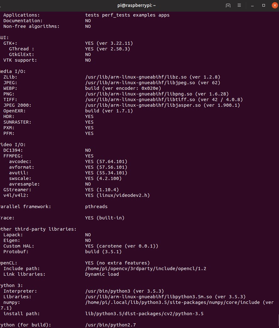 It should be noted that the above library compilation procedure must be performed both on the robot and on the PC from which it is planned to control the robot and on which broadcasts from the robot will be received.Creating a video distribution schemeBefore you start writing code, you need to develop a scheme according to which the algorithm will function. In the considered case of software development for a robot created for participation in the RTK Cup competitions in the Extreme nomination, the entire program will be divided into two parts: a robot and a remote control, which will be played by a computer with Linux installed. One of the most important tasks here is to create an approximate scheme of how video data will be transmitted between different parts of the algorithm. Wi-Fi will be used as a communication channel between the two devices. Data packets providing control of the robot and feedback data will be transmitted from one device to another using the UDP protocol implemented in using the socket library. Video datadue to limitations in the size of the UDP packet will be transmitted using GStreamer. For the convenience of debugging, two video streams will be implemented:
- main video stream - transfers video data directly from the robot’s camera to a computer to ensure minimal control delay.
- auxiliary video stream - transfers the video data processed by the robot, necessary for setting up and debugging a program that implements computer vision.
Two video streams will be simultaneously active on the robot, and the computer will display the desired image depending on the drive mode enabled. The robot, in turn, depending on whether the autonomy mode is on or off, will use either control data received from a computer or generated by an image processor. Remote control of the robot will be carried out due to the work of two parallel flows on the robot and on the computer:
- The “console” in a cycle polls all available input devices and forms a control data packet consisting of the data itself and the checksum (at the time of making the final changes to the article, I refused to create checksums in order to reduce the delay, but in the source, which I laid out at the end this piece of code is left) - of a certain value calculated from a data set by the operation of some algorithm used to determine the integrity of data during transmission
- Robot - Awaits data access from the computer. Unpacks the data, recalculates the checksum and compares it with the sent and calculated on the computer side. If the checksums match, the data is transferred to the main program.
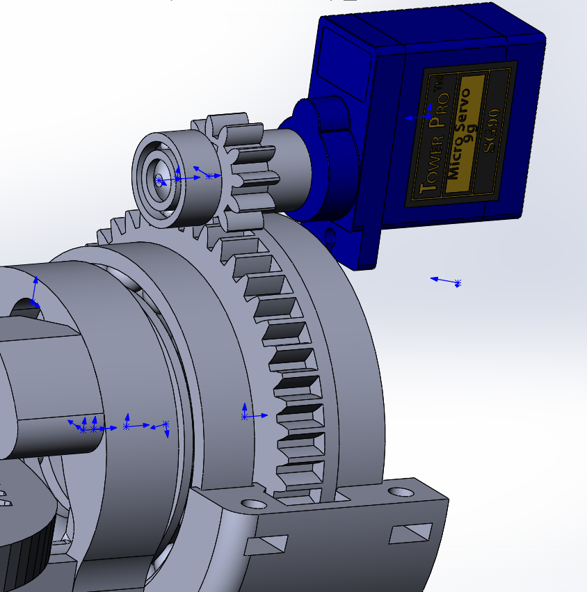
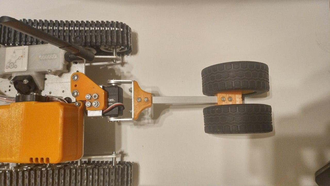
Before parsing the line detection algorithm, I suggest that you familiarize yourself with the design features of the robot:about the robot.
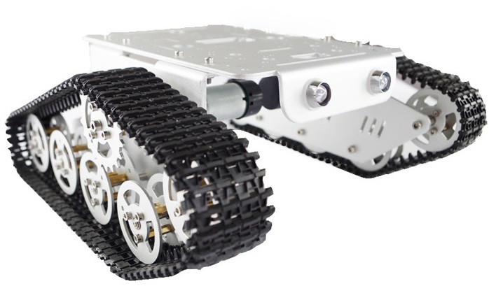
— . (3 ) . , . 6 , . . . . , - . «» rasberry pi 3 b — .
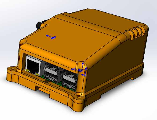
, , , , Solidworks petg . , raspberry .

ubiquiti bullet M5 hp. ( ) , . , «»
.
: «»
thingiverse. , , , , .
, , . , . , , , , . , , , .
- ( - 200 ) , , 90 70 ( ), , « ». , VL53L0X , .
«» , , (
rds3115). — , , , , .
, , , :
- , , , . .
raspberry, , . , .
, USB. , , .
Creation of a line detection algorithm using OpenCV library methods
I. Receiving data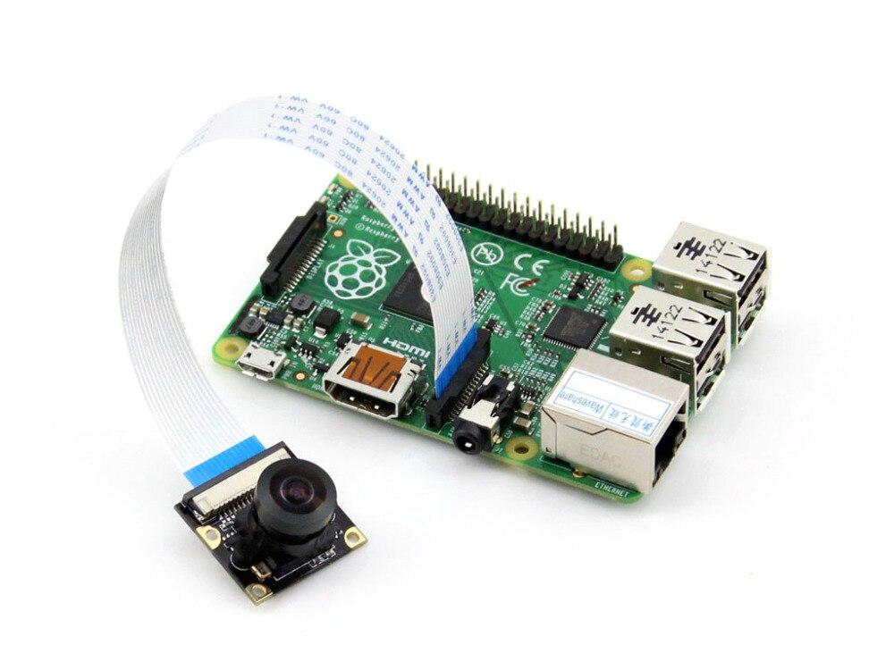 Due to the fact that the image processor does not receive video data directly from the camera, but from the main stream, it is necessary to transfer them from the format used for translation to the format used for image processing, namely, a numpy array consisting of red values , green and blue for each of the pixels. To do this, you need the initial data - a frame received from the raspberry pi camera module.The easiest way to get frames from camera c for further processing is to use the picamera library. Before you begin, you need to allow access to the camera through raspi-config -> interfacing options camera -> select yes.
sudo raspi-config
the next section of code is connected to the raspberry camera and in a cycle with a given frequency receives frames in the form of an array ready for use by the opencv library.from picamera.array import PiRGBArray
from picamera import PiCamera
import cv2
camera = PiCamera()
camera.resolution = (640, 480)
camera.framerate = 30
cap = PiRGBArray(camera, size=(640, 480))
for frame in camera.capture_continuous(cap , format="bgr", use_video_port=True):
new_frame = frame.array
cap.truncate(0)
if False:
break
It is also worth noting that this method of capturing frames, although it is the simplest, but has a serious drawback: it is not very effective if you need to broadcast frames through GStreamer, as this requires several times to re-encode the video, which reduces the speed of the program. A much faster way to obtain images will be to output frames from the video stream at the request of the image processor, however, the further stages of image processing will not depend on the method used.An example of an image from a robot heading camera without processing:II. Pre-processingWhen driving on a line, it will be most simple to separate the area of points that most contrast with the background color. This method is ideally suited for the RTK Cup competition, because it uses a black line on a white background (or a white line on a black background for inverse sections). In order to reduce the amount of information that needs to be processed, you can apply a binarization algorithm to it, that is, convert the image to a monochrome format, where there are only two types of pixels - dark and light. Before this, the picture should be translated into grayscale, and also blur it in order to cut off small defects and noise that inevitably appears during the operation of the camera. To blur the image, a Gaussian filter is used.gray = cv2.cvtColor(self._frame, cv2.COLOR_RGB2GRAY)
blur = cv2.GaussianBlur(gray, (ksize, ksize), 0)
where ksize is the size of the Gaussian core, increasing which, you can increase the degree of blur.Example image after translation in grayscale and blur:III. Selecting detailsAfter the image is translated in grayscale, it is necessary to binarize it at a given threshold. This action allows you to further reduce the amount of data. This threshold value will be adjusted before each departure of the robot in a new place, or when the lighting conditions change. Ideally, the task of calibration is to make sure that the outline of the line is defined on the image, but at the same time, there should not be other details on the image that are not a line:thresh = cv2.threshold(blur, self._limit, 255, cv2.THRESH_BINARY_INV)[1]
Here, all pixels darker than the threshold value (self._limit) are replaced by 0 (black), lighter - by 255 (white).After processing, the image looks as follows:As you can see, the program has identified several of the darkest parts of the image. However, having calibrated the threshold value so as to completely “catch” the headphones, other white elements appear on the screen besides them. Of course, you can fine-tune the threshold, and at the competitive training ground the camera will look down, not allowing unnecessary elements into the frame, but I consider it necessary for me to separate the line from everything else.IV.DetectionIn the binarized image, I applied a border search algorithm. It is needed in order to determine free-standing spots and turn them into a convenient array of coordinate values of points that make up the border. In the case of opencv, as written in the documentation, the standard algorithm for finding loops uses the Suzuki85 algorithm (I could not find references to the algorithm with this name anywhere except for the opencv documentation, but I will assume that this is the Suzuki-Abe algorithm ).contours = cv2.findContours(thresh, cv2.RETR_TREE, cv2.CHAIN_APPROX_SIMPLE)[0]
And here is the frame obtained at this stage:V. High Level ProcessingHaving found all the contours in the frame, the contour with the largest area is selected and taken as the contour of the line. Knowing the coordinates of all points of this contour, the coordinate of its center is found. For this, the so-called "image moments" are used. The moment is the total characteristic of the contour, calculated by summing the coordinates of all the pixels of the contour. There are several types of moments - up to the third order. For this problem, only the zero-order moment (m00) is needed - the number of all points making up the contour (the perimeter of the contour), the first-order moment (m10), which is the sum of X coordinates of all points, and m01 is the sum of Y coordinates of all points. By dividing the sum of the coordinates of the points along one of the axes by their number, the arithmetic mean is obtained — the approximate coordinate of the center of the contour. Next, the deviation of the robot from the course is calculated:the course “directly” corresponds to the coordinate of the center point along X close to the frame width divided by two. If the coordinate of the center of the line is close to the center of the frame, then the control action is minimal, and, accordingly, the robot retains its current course. If the robot deviates from one of the sides, then a control action proportional to the deviation will be introduced until it returns.mainContour = max(contours, key = cv2.contourArea)
M = cv2.moments(mainContour)
if M['m00'] != 0:
cx = int(M['m10']/M['m00'])
cy = int(M['m01']/M['m00'])
Below is a schematic drawing of the position of the robot relative to the line and the frames, with the results of the program superimposed on them: the “main” contour, the lines passing through the center of the contour, as well as the point located in the center to estimate the deviation. These elements are added using the following code:cv2.line(frame, (cx, 0), (cx, self.height), (255, 0, 0), 1)
cv2.line(frame, (0, cy), (self.width, cy), (255, 0, 0), 1)
cv2.circle(frame, (self.width//2, self.height//2), 3, (0, 0, 255), -1)
cv2.drawContours(frame, mainContour, -1, (0, 255, 0), 2, cv2.FILLED)
For convenience of debugging, all previously described elements are added to the raw frame: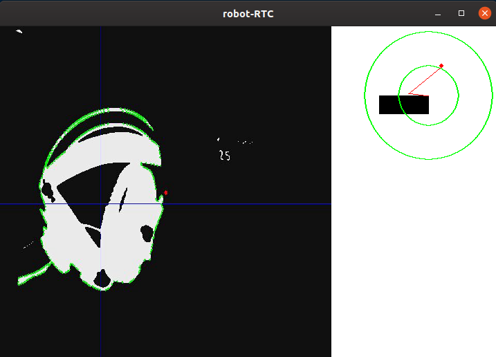
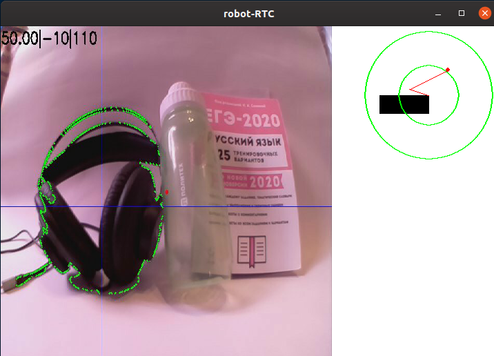 Thus, having driven the frame through the processing algorithm, we got the X and Y coordinates of the center of the object of interest to us, as well as the debug image. Next, the position of the robot relative to the line is schematically shown, as well as the image that has passed the processing algorithm.The next step in the program is to convert the information obtained in the previous step into the power values of two motors.
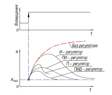 The easiest way to convert the difference between the shift of the center of the color spot relative to the center of the frame is the proportional regulator (There is also a relay regulator, but, due to the features of its operation, it is not very suitable for driving along the line). The principle of operation of such an algorithm is that the controller generates a control action on the object in proportion to the magnitude of the error. In addition to the proportional controller, there is also an integral one, where over time the integral component “accumulates” the error and the differential ones, the principle of which is based on the application of the regulatory influence only with a sufficient change in the controlled variable. In practice, these simplest P, I, D controllers are combined into controllers of the type PI, PD, PID.It is worth mentioning that on my robot I tried to “start” the PID controller, but its use did not give any serious advantages over the usual proportional controller. I admit that I could not properly adjust the regulator, but it is also possible that its advantages are not so clearly visible in the case of a heavy robot that is unable to physically develop high speeds. In the latest version of the program at the time of writing, a simple proportional regulator is used, but with a small feature that allows you to use more information from the camera: when generating the error value, not only the horizontal position of the midpoint of the spot was taken into account, but also vertically, which allowed different ways respond to line elementslocated “in the distance” and directly in front of or under the robot (the robot’s heading camera has a huge viewing angle, so turning it just 45 degrees down, you can already see a significant part of the field under the robot).
error= cx / (self.width/2) - 1
error*= cy / self.height + self.gain
Most often, in the conditions of the “RTK Cup” competition, the participants use the so-called “tank circuit” - one or more engines control one side of the robot, and it works both with tracks and with wheels. Using this scheme allows you to get rid of complex transmission elements that increase the chance of breakage (differentials or cardan shafts), get the smallest possible turning radius, which gives an advantage in a confined polygon. This scheme involves the parallel control of two “sides” for movement along a complex path. To do this, the program uses two variables - the power of the right and left motor. This power depends on the base speed (BASE_SPEED), varying in the range from 0 to 100.Errors (error) - the difference between the center of the frame and the coordinate of the middle of the line and the coefficient of proportional effect (self._koof), which is calibrated by the operator. Its absolute value affects how fast the robot will try to align itself with the line. Due to the fact that on one engine the control action is subtracted from the base speed, and on the other - it is added, a turn is carried out when deviating from the course. The direction in which the reversal will be performed can be adjusted by changing the sign of the self._koof variable. Also, you may notice that as a result of the next code section, a power value may appear that is more than 100, but in my program such cases are additionally processed later.Its absolute value affects how fast the robot will try to align itself with the line. Due to the fact that on one engine the control action is subtracted from the base speed, and on the other - it is added, a turn is carried out when deviating from the course. The direction in which the reversal will be performed can be adjusted by changing the sign of the self._koof variable. Also, you may notice that as a result of the next code section, a power value may appear that is more than 100, but in my program such cases are additionally processed later.Its absolute value affects how fast the robot will try to align itself with the line. Due to the fact that on one engine the control action is subtracted from the base speed, and on the other - it is added, a turn is carried out when deviating from the course. The direction in which the reversal will be performed can be adjusted by changing the sign of the self._koof variable. Also, you may notice that as a result of the next code section, a power value may appear that is more than 100, but in my program such cases are additionally processed later.in which the reversal will be made, you can adjust by changing the sign of the self._koof variable. Also, you may notice that as a result of the next code section, a power value may appear that is more than 100, but in my program such cases are additionally processed later.in which the reversal will be made, you can adjust by changing the sign of the self._koof variable. Also, you may notice that as a result of the next code section, a power value may appear that is more than 100, but in my program such cases are additionally processed later.
leftSpeed = round(self.base_speed + error*self.koof)
rightSpeed = round(self.base_speed - error*self.koof)
Conclusion
Having tested the resulting program, I can say that the main difficult moment in setting up the program is the calibration of the algorithm to the lighting features. Since the stage of creating the article coincided with the declared self-isolation, I had to create a video with a demonstration of work in a small room. This put the following difficulties on me:- -, , ( , ), . , , , . , , , ,
- -, — , ,
Despite the fact that both of these problems are absent in the conditions of real competitions, I will take measures to ensure that the work of the program minimally depends on external factors.Also, in the future, it is planned to continue work on the implementation of algorithms using computer vision methods, creating software capable of passing through the remaining elements of autonomy described in the first part of the article (autonomous beacon capture, movement along a complex path). It is planned to expand the functionality of the robot by adding additional sensors: rangefinder, gyroscope-accelerometer, compass. Despite the fact that the publication of this article will end my work on the project as a compulsory school subject, I plan to continue to describe here the further stages of development. Therefore, I would like to receive comments about this work.After implementing all the steps aimed at solving the problems of the project, it is safe to say that the use of computer vision algorithms, with all its relative complexity in programming and debugging, gives the greatest gain at the stage of the competitions themselves. With the small dimensions of the camera, it has enormous potential in terms of software development, because the camera allows you to replace several "traditional" sensors at once, while receiving incredibly more information from the outside world. It was possible to realize the goal of the project - to create a program that uses computer vision to solve the problem of autonomous navigation of the robot in the conditions of the “RTK Cup” competition, as well as describe the process of creating the program and the main stages in image processing.As I said earlier, it was not possible to recreate the complex trajectory of the house line, however, and this example shows how the algorithm fulfills turns. The thickness of the line here corresponds to that according to the regulations, and the most curve of the turns approximately reflects the curvature of rotation by 90 degrees on the polygon:You can see the program code, as well as monitor further work on the project, on my github or here, if I continue.