F #, marking algorithm for connected image components

Search and marking of connected components in binary images is one of the basic algorithms for image analysis and processing. In particular, this algorithm can be used in machine vision to search and count common structures in the image, with their subsequent analysis.

In the framework of this article, two algorithms for marking connected components will be considered, their implementation in the programming language F # is shown. And also, a comparative analysis of the algorithms, the search for weaknesses. The source material for the implementation of the algorithms was taken from the book “ Computer Vision” (authors L. Shapiro, J. Stockman. Translation from English by A. A. Boguslavsky edited by S. M. Sokolov) .

Introduction

A connected component with a value of v is a set of C such pixels that have a value of v and each pair of these pixels is connected with a value of v

It sounds abstruse, so let's just see the picture. We assume that the foreground pixels of the binary image are marked as 1 , and the background pixels are marked as 0 .

After processing the image with the marking algorithm of the connected components, we get the following picture. Here, instead of pixels, connected components are formed, which differ from each other in number. In this example, 5 components were found and it will be possible to work with them as with separate entities.

Figure 1: Labeled Connected Components

$$

$$\begin{matrix} 1 & 1 & 0 & 1 & 1 & 1 & 0 & 2 \\ 1 & 1 & 0 & 1 & 0 & 1 & 0 & 2 \\ 1 & 1 & 1 & 1 & 0 & 0 & 0 & 2 \\ 0 & 0 & 0 & 0 & 0 & 0 & 0 & 2 \\ 3 & 3 & 3 & 3 & 0 & 4 & 0 & 2 \\ 0 & 0 & 0 & 3 & 0 & 4 & 0 & 2 \\ 5 & 5 & 0 & 3 & 0 & 0 & 0 & 2 \\ 5 & 5 & 0 & 3 & 0 & 2 & 2 & 2 \end{matrix}$$

Two algorithms that can be used to solve such a problem will be considered below.

Recursive labeling algorithm

We will start by looking at the recursion-based algorithm as the most obvious. The principle of operation of such an algorithm will be as follows.

Assign a label, which we will mark related components, the initial value.

1. We sort through all the points in the table, starting with the coordinate 0x0 (upper left corner). After processing the next point, increase the label by one
2. If the pixel at the current coordinate is 1 , then we scan all four neighbors of this point (top, bottom, right, left)
3. If the neighboring point is also 1 , then the function recursively calls itself to process the neighbor until it hits the boundary of the array or point 0
4. During the recursive processing of the neighbor, a check must be made that the point has not already been processed and is marked with the current marker.

Thus, sorting through all the points in the array and invoking a recursive algorithm for each, then at the end of the search we get a fully marked table. Since there is a check on whether a given point has already been marked, each point will be processed only once. The recursion depth will depend only on the number of connected neighbors to the current point. This algorithm is well suited for images that do not have a large image fill. That is, images in which there are thin and short lines, and everything else is a background image that is not processed. Moreover, the speed of such an algorithm may be higher than the line-by-line algorithm (we will discuss it later in the article).

Since two-dimensional binary images are two-dimensional matrices, when writing the algorithm, I will operate with the concepts of matrices, about which I made a separate article, which can be read here.

Functional programming using the example of working with matrices from the theory of linear algebra.

Let us consider and analyze in detail the F # -function that implements recursive labeling algorithm for connected binary image components

let recMarkingOfConnectedComponents matrix =

        let copy = Matrix.clone matrix

        let (|Value|Zero|Out|) (x, y) = 
            if x < 0 || y < 0
                || x > (copy.values.[0, *].Length - 1)
                || y > (copy.values.[*, 0].Length - 1) then
                Out
            else
                let row = copy.values.[y, *]
                match row.[x] with
                    | 0 -> Zero
                    | v -> Value(v)

        let rec markBits x y value =
            match (x, y) with
            | Value(v) ->
                if value > v then
                    copy.values.[y, x] <- value
                    markBits (x + 1) y value
                    markBits (x - 1) y value
                    markBits x (y + 1) value
                    markBits x (y - 1) value
            | Zero | Out -> ()

        let mutable value = 2
        copy.values
        |> Array2D.iteri (fun y x v -> if v = 1 then
                                            markBits x y value
                                            value <- value + 1)

        copy 

We declare the recMarkingOfConnectedComponents function , which takes a two-dimensional array of matrix, packed into a record of type Matrix. The function will not change the original array, so first create a copy of it, which will be processed by the algorithm and returned.

let copy = Matrix.clone matrix

To simplify the checks of the indices of the requested points outside the array, create an active template that returns one of three values.

Out - the requested index went beyond the two-dimensional array
Zero - the point contains a background pixel (equal to zero)
Value - the requested index is within the array

This template will simplify checking the coordinates of the image point at the next recursion frame:

let (|Value|Zero|Out|) (x, y) = 
    if x < 0 || y < 0
        || x > (copy.values.[0, *].Length - 1)
        || y > (copy.values.[*, 0].Length - 1) then
        Out
    else
        let row = copy.values.[y, *]
        match row.[x] with
            | 0 -> Zero
            | v -> Value(v)

The MarkBits function is declared recursive and serves to process the current pixel and all its neighbors (top, bottom, left, right):

let rec markBits x y value =
    match (x, y) with
    | Value(v) ->
        if value > v then
            copy.values.[y, x] <- value
            markBits (x + 1) y value
            markBits (x - 1) y value
            markBits x (y + 1) value
            markBits x (y - 1) value
    | Zero | Out -> ()

The function accepts the following parameters as an input:

x - row number
y - column number
value - current label value to mark the pixel

Using the match / with construct and the active template (above), the pixel coordinates are checked so that it does not go beyond the two-dimensional array. If the point is inside a two-dimensional array, then we do a preliminary check so as not to process the point that has already been processed.

if value > v then

Otherwise, infinite recursion will occur and the algorithm will not work.

Next, mark the point with the current marker value:

copy.values.[y, x] <- value

And we process all its neighbors, recursively calling the same function:

markBits (x + 1) y value
markBits (x - 1) y value
markBits x (y + 1) value
markBits x (y - 1) value

After we implemented the algorithm, it must be used. Consider the code in more detail.

let mutable value = 2
copy.values
|> Array2D.iteri (fun y x v -> if v = 1 then
                                    markBits x y value
                                    value <- value + 1) 

Before processing the image, set the initial value of the label, which will mark the connected groups of pixels.

let mutable value = 2

The fact is that the front pixels in the binary image are already set to 1 , so if the initial value of the label is also 1 , then the algorithm will not work. Therefore, the initial value of the label must be greater than 1 . There is another way to solve the problem. Before starting the algorithm, mark all pixels set to 1 with an initial value of -1 . Then we can set the value to 1 . You can do it yourself if you want.

The next construction, using the Array2D.iteri function, iterates over all the points in the array, and if during the search you encounter a point set to 1, then this means that it is not processed and for it you need to call the recursive function markBits with the current label value. All pixels set to 0 are ignored by the algorithm.

After recursively processing the point, we can assume that the entire connected group to which this point belongs is guaranteed to be marked and you can increase the label value by 1 to apply it to the next connected point.

Consider an example of the application of such an algorithm.

let a = array2D [[1;1;0;1;1;1;0;1]
                 [1;1;0;1;0;1;0;1]
                 [1;1;1;1;0;0;0;1]
                 [0;0;0;0;0;0;0;1]
                 [1;1;1;1;0;1;0;1]
                 [0;0;0;1;0;1;0;1]
                 [1;1;0;1;0;0;0;1]
                 [1;1;0;1;0;1;1;1]]
let A = Matrix.ofArray2D a

let t = System.Diagnostics.Stopwatch.StartNew()
let R = Algorithms.recMarkingOfConnectedComponents A
t.Stop()

printfn "origin =\n %A" A.values
printfn "rec markers =\n %A" R.values
printfn "elapsed recurcive = %O" t.Elapsed 

origin =
 [[1; 1; 0; 1; 1; 1; 0; 1]
 [1; 1; 0; 1; 0; 1; 0; 1]
 [1; 1; 1; 1; 0; 0; 0; 1]
 [0; 0; 0; 0; 0; 0; 0; 1]
 [1; 1; 1; 1; 0; 1; 0; 1]
 [0; 0; 0; 1; 0; 1; 0; 1]
 [1; 1; 0; 1; 0; 0; 0; 1]
 [1; 1; 0; 1; 0; 1; 1; 1]]

rec markers =
 [[2; 2; 0; 2; 2; 2; 0; 3]
 [2; 2; 0; 2; 0; 2; 0; 3]
 [2; 2; 2; 2; 0; 0; 0; 3]
 [0; 0; 0; 0; 0; 0; 0; 3]
 [4; 4; 4; 4; 0; 5; 0; 3]
 [0; 0; 0; 4; 0; 5; 0; 3]
 [6; 6; 0; 4; 0; 0; 0; 3]
 [6; 6; 0; 4; 0; 3; 3; 3]]

elapsed recurcive = 00:00:00.0037342

The advantages of a recursive algorithm include its simplicity in writing and understanding. It is great for binary images containing a large background and interspersed with small groups of pixels (for example, lines, small spots, and so on). In this case, the image processing speed may be high, since the algorithm processes the entire image in one pass.

The disadvantages are also obvious - this is recursion. If the image consists of large spots or is completely flooded, then the processing speed drops sharply (by orders of magnitude) and there is a risk that the program will crash at all due to lack of free space on the stack.

Unfortunately, the tail recursion principle cannot be applied in this algorithm, because tail recursion has two requirements:

1. Each recursion frame must perform calculations and add the result to the accumulator, which will be transmitted down the stack.
2. There should not be more than one recursive function call in one recursion frame.

In our case, recursion does not perform any final calculations, which can be passed to the next frame of recursion, but simply modifies a two-dimensional array. In principle, this could be circumvented by simply returning a single number, which in itself does not mean anything. We also make 4 calls recursively, since we need to process all four neighbors of the point.

Classical algorithm for marking connected components based on data structure to combine searches

The algorithm also has another name, “Algorithm of progressive marking,” and here we will try to parse it.

. . . , , .

The definition above is even more confusing, so we will try to deal with the principle of the algorithm in a different way and start from afar.

First, we will deal with the definition of a four - connected and eight-connected neighborhood of the current point. Look at the pictures below to understand what it is and what is the difference.

Figure 2: The four-connected component
\ begin {matrix} Figure 2: The eight-connected component \ begin {matrix} The first picture shows a four-connected component $$\begin{matrix} & 1 & \\ 2 & * & 3 \\ & 4 & \end{matrix}$$


$$\begin{matrix} 1 & 2 & 3 \\ 4 & * & 5 \\ 6 & 7 & 8 \end{matrix}$$
points, that is, this means that the algorithm processes 4 neighbors of the current point (left, right, top and bottom). Accordingly, the eight-connected component of a point means that it has 8 neighbors. In this article, we will work with four-connected components.

Now you need to figure out what is a data structure for combining search , built on some sets?

For example, suppose we have two sets

$$

$$(1, 2, 3, 4, 8) (5, 6, 7)$$

These sets are organized in the form of the following trees: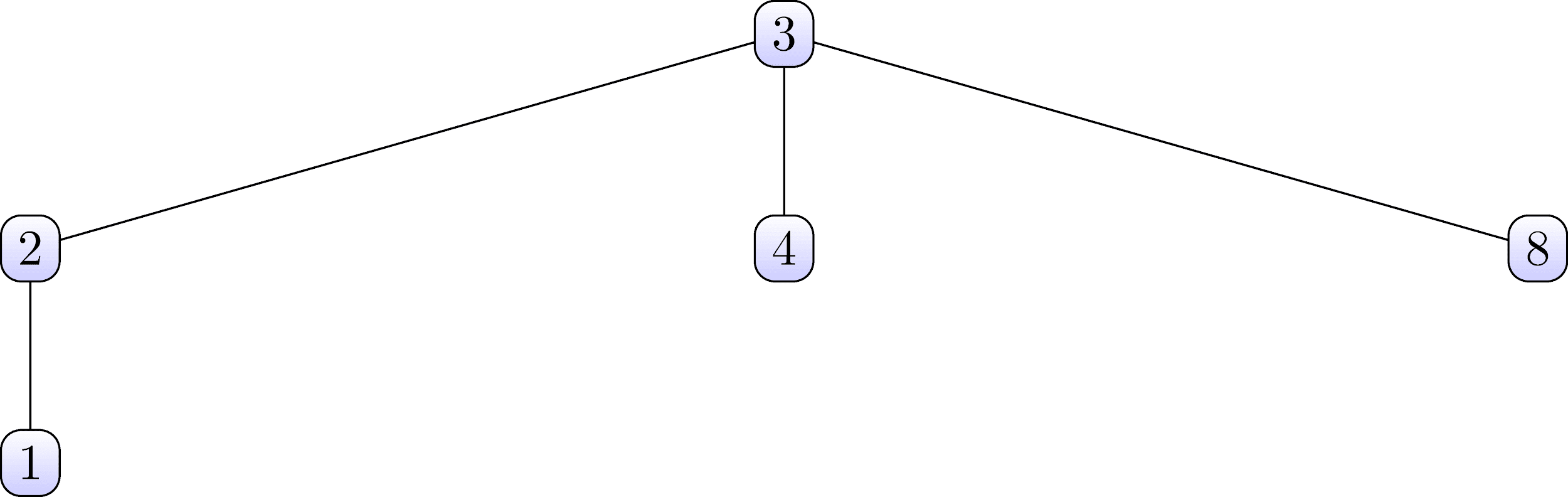





Note that in the first set, nodes 3 are root, and in the second, nodes 6.

Now we consider the data structure for a search-union, which contains both of these sets, and also organizes their tree structure .

Figure 4: Data structure for search-union
\ begin {matrix} Look carefully at the table above and try to find a relationship with the set trees shown above. The table should be viewed in vertical columns. It is seen,that the number 3 in the first line corresponds to the number 0 $$\begin{matrix} 1 & 2 & 3 & 4 & 5 & 6 & 7 & 8 \\ 2 & 3 & 0 & 3 & 7 & 7 & 0 & 3 \end{matrix}$$

in the second line. And in the first tree, the number 3 is the root of the first set. By analogy, you can find that the number 7 from the first line corresponds to the number 0 from the second line. The number 7 is also the root of the tree of the second set.

Thus, we conclude that the numbers from the upper row are the daughter nodes of the sets, and the corresponding numbers from the lower row are their parent nodes. Guided by this rule, you can easily restore both trees from the above table.

We analyze such details so that later it will be easier for us to understand how the progressive marking algorithm works.. For now, let’s dwell on the fact that a series of numbers from the first row is always numbers from 1 to a certain maximum number. In fact, the maximum number of the first row is the maximum value of the labels with which the found connected components will be marked . And individual sets are transitions between labels that are formed as a result of the first pass (we will consider in more detail later).

Before proceeding, consider the pseudo-code of some functions that will be used by the algorithm.

We denote the table representing the data structure for the join-search as PARENT . The next function is called find and will take the current label X as parametersand an array of PARENT . This procedure traces parent pointers up to the root of the tree and finds the label of the root node of the tree to which X belongs .

 ̆   ̆  .
X —  
PARENT — , ̆    -

procedure find(X, PARENT);
{
j := X;
while PARENT[j] <> 0
    j := PARENT[j]; return(j);
}

Consider how such a function can be implemented on F #

let rec find x =
    let index = Array.tryFindIndex ((=)x) parents.[0, *]
    match index with
    | Some(i) -> 
        match parents.[1, i] with
        | p when p <> 0 -> find p
        | _ -> x
    | None -> x 

Here we declare a recursive function of the find , which takes the current label the X . The PARRENT array is not passed here, since we already have it in the global namespace and the function already sees it and can work with it.

First, the function tries to find the index of the label on the top line (since you need to find its parent, which is located on the bottom line.

let index = Array.tryFindIndex ((=)x) parents.[0, *]

If the search succeeds, then we get its parent and compare with 0 . If the parent is not 0 , then this node also has a parent and the function recursively calls itself until the parent is 0 . This will mean that we have found the root node of the set.

match index with
    | Some(i) -> 
        match parents.[1, i] with
        | p when p <> 0 -> find p
        | _ -> x
    | None -> x 

The next function we need is called union . It takes two labels X and Y , as well as an array of PARENT . This structure modifies (if necessary) PARENT fusion subset containing a label X , with the set comprising label Y . The procedure searches for the root nodes of both labels and if they do not match, then the node of one of the labels is designated as the parent node of the second label. So there is a union of two sets.

   .
X — ,   .
Y — ,   .
PARENT — , ̆    -.

procedure union(X, Y, PARENT);
{
j := X;
k := Y;
while PARENT[j] <> 0
    j := PARENT[j];
while PARENT[k]] <> 0
    k := PARENT[k];

if j <> k then PARENT[k] := j;
} 

F # implementation looks like this

let union x y =
    let j = find x
    let k = find y
    if j <> k then parents.[1, k-1] <- j 

Note that the find function we have already implemented is already used here .

The algorithm also requires two additional functions, which are called neighbors and labels . The neighbors function returns the set of neighboring points to the left and top (since in our case the algorithm works on a four-connected component) from the given pixel, and the labels function returns the set of labels that were already assigned to the given set of pixels that the neighbors function returned . In our case, we will not implement these two functions, but we will make only one that combines both functions and returns the found labels.

let neighbors_labels x y =
    match (x, y) with
    | (0, 0) -> []
    | (0, _) -> [step1.[0, y-1]]
    | (_, 0) -> [step1.[x-1, 0]]
    | _ -> [step1.[x, y-1]; step1.[x-1, y]]
    |> List.filter ((<>)0) 

Looking ahead, I’ll say right away that the array step1 that uses the function already exists in the global space and contains the result of processing the algorithm on the first pass. I want to pay special attention to the additional filter.

|> List.filter ((<>)0)

It cuts off all results that are 0 . That is, if the label contains 0 , then we are dealing with a point in the background image that does not need to be processed. This is a very important nuance that is not mentioned in the book from which we take examples, but nevertheless, the algorithm will not work without such a check.

Gradually, step by step, we get closer to the very essence of the algorithm. Let's look again at the image that we will need to process.

Figure 5: Original binary image
\ begin {matrix} $$\begin{matrix} 1 & 1 & 0 & 1 & 1 & 1 & 0 & 1 \\ 1 & 1 & 0 & 1 & 0 & 1 & 0 & 1 \\ 1 & 1 & 1 & 1 & 0 & 0 & 0 & 1 \\ 0 & 0 & 0 & 0 & 0 & 0 & 0 & 1 \\ 1 & 1 & 1 & 1 & 0 & 1 & 0 & 1 \\ 0 & 0 & 0 & 1 & 0 & 1 & 0 & 1 \\ 1 & 1 & 0 & 1 & 0 & 0 & 0 & 1 \\ 1 & 1 & 0 & 1 & 0 & 1 & 1 & 1 \end{matrix}$$

Before processing, create an empty array step1 , in which the result of the first pass will be saved.

Figure 6: Array step1 for storing the primary processing results
\ begin {matrix} $$\begin{matrix} 0 & 0 & 0 & 0 & 0 & 0 & 0 & 0 \\ 0 & 0 & 0 & 0 & 0 & 0 & 0 & 0 \\ 0 & 0 & 0 & 0 & 0 & 0 & 0 & 0 \\ 0 & 0 & 0 & 0 & 0 & 0 & 0 & 0 \\ 0 & 0 & 0 & 0 & 0 & 0 & 0 & 0 \\ 0 & 0 & 0 & 0 & 0 & 0 & 0 & 0 \\ 0 & 0 & 0 & 0 & 0 & 0 & 0 & 0 \\ 0 & 0 & 0 & 0 & 0 & 0 & 0 & 0 \end{matrix}$$

Consider the first few steps of the primary data processing (only the first three lines of the original binary image).

Before we take a step-by-step look at the algorithm, let's look at the pseudo-code that explains the general principle of operation.

     .
B —   .
LB —   .

procedure classical_with_union-find(B, LB);
{
“  .” initialize();
“  1 ̆  L     .”
for L := 0 to MaxRow
{
“     L  ”
for P := 0 to MaxCol
    LB[L,P] := 0;
“  L.”
for P := 0 to MaxCol
    if B[L,P] == 1 then
    {
        A := prior_neighbors(L,P);
        if isempty(A)
        then {M := label; label := label + 1;};
        else M := min(labels(A));
        LB[L,P] := M;
        for X in labels(A) and X <> M
           union(M, X, PARENT);
    }
}
“  2 ,    1,     .”
for L := 0 to MaxRow
    for P := 0 to MaxCol
        if B[L, P] == 1
        then LB[L,P] := find(LB[L,P], PARENT);
};
      LB ( step1)     ( ).

Figure 7: Step 1. Point (0,0), label = 1
\ begin {matrix} Figure 8: Step 2. Point (1,0), label = 1 \ begin {matrix} Figure 9: Step 2. Point (2,0), label = 1 \ begin {matrix} Figure 10: Step 4. Point (3.0), label = 2 \ begin {matrix} $$\begin{matrix} 1 & 0 & 0 & 0 & 0 & 0 & 0 & 0 \\ 0 & 0 & 0 & 0 & 0 & 0 & 0 & 0 \\ 0 & 0 & 0 & 0 & 0 & 0 & 0 & 0 \end{matrix}$$

$$\begin{matrix} 1 & 1 & 0 & 0 & 0 & 0 & 0 & 0 \\ 0 & 0 & 0 & 0 & 0 & 0 & 0 & 0 \\ 0 & 0 & 0 & 0 & 0 & 0 & 0 & 0 \end{matrix}$$

$$\begin{matrix} 1 & 1 & 0 & 0 & 0 & 0 & 0 & 0 \\ 0 & 0 & 0 & 0 & 0 & 0 & 0 & 0 \\ 0 & 0 & 0 & 0 & 0 & 0 & 0 & 0 \end{matrix}$$

$$\begin{matrix} 1 & 1 & 0 & 2 & 0 & 0 & 0 & 0 \\ 0 & 0 & 0 & 0 & 0 & 0 & 0 & 0 \\ 0 & 0 & 0 & 0 & 0 & 0 & 0 & 0 \end{matrix}$$
Figure 11: Last step, final result of the first pass
\ begin { matrix} Note that as a result of the initial processing of the original image, we got two sets $$\begin{matrix} 1 & 1 & 0 & 2 & 2 & 2 & 0 & 3 \\ 1 & 1 & 0 & 2 & 0 & 2 & 0 & 3 \\ 1 & 1 & 1 & 1 & 0 & 0 & 0 & 3 \\ 0 & 0 & 0 & 0 & 0 & 0 & 0 & 3 \\ 4 & 4 & 4 & 4 & 0 & 5 & 0 & 3 \\ 0 & 0 & 0 & 4 & 0 & 5 & 0 & 3 \\ 6 & 6 & 0 & 4 & 0 & 0 & 0 & 3 \\ 6 & 6 & 0 & 4 & 0 & 7 & 7 & 3 \end{matrix}$$

$$

$$(1,2) - (3,7)$$

Visually, this can be seen as the contact of marks 1 and 2 (coordinates of points (1,3) and (2,3) ) and marks 3 and 7 (coordinates of points (7,7) and (7,6) ). From the point of view of the data structure for search-union, this result is obtained.

Figure 12: The calculated data structure for joining the search
\ begin {matrix} After finally image processing using the obtained data structure, we obtain the following result. Figure 13:Final result \ begin {matrix} $$\begin{matrix} 1 & 2 & 3 & 4 & 5 & 6 & 7 \\ 0 & 1 & 0 & 0 & 0 & 0 & 3 \end{matrix}$$



$$\begin{matrix} 1 & 1 & 0 & 1 & 1 & 1 & 0 & 3 \\ 1 & 1 & 0 & 1 & 0 & 1 & 0 & 3 \\ 1 & 1 & 1 & 1 & 0 & 0 & 0 & 3 \\ 0 & 0 & 0 & 0 & 0 & 0 & 0 & 3 \\ 4 & 4 & 4 & 4 & 0 & 5 & 0 & 3 \\ 0 & 0 & 0 & 4 & 0 & 5 & 0 & 3 \\ 6 & 6 & 0 & 4 & 0 & 0 & 0 & 3 \\ 6 & 6 & 0 & 4 & 0 & 3 & 3 & 3 \end{matrix}$$
Now all the connected components we have have unique labels and their can be used in subsequent algorithms for processing.

The F # code implementation is as follows

let markingOfConnectedComponents matrix =

    // up to 10 markers
    let parents = Array2D.init 2 10 (fun x y -> if x = 0 then y+1 else 0)

    // create a zero initialized copy
    let step1 = (Matrix.cloneO matrix).values

    let rec find x =
        let index = Array.tryFindIndex ((=)x) parents.[0, *]
        match index with
        | Some(i) -> 
            match parents.[1, i] with
            | p when p <> 0 -> find p
            | _ -> x
        | None -> x

    let union x y =
        let j = find x
        let k = find y
        if j <> k then parents.[1, k-1] <- j

    // returns up and left neighbors of pixel
    let neighbors_labels x y =
        match (x, y) with
        | (0, 0) -> []
        | (0, _) -> [step1.[0, y-1]]
        | (_, 0) -> [step1.[x-1, 0]]
        | _ -> [step1.[x, y-1]; step1.[x-1, y]]
        |> List.filter ((<>)0)

    let mutable label = 0
    matrix.values
    |> Array2D.iteri (fun x y v ->
                        if v = 1 then
                            let n = neighbors_labels x y
                            let m = if n.IsEmpty then
                                        label <- label + 1
                                        label
                                    else
                                        n |> List.min
                            n |> List.iter (fun v -> if v <> m then union m v)
                            step1.[x, y] <- m)

    let step2 = matrix.values
                |> Array2D.mapi (fun x y v ->
                        if v = 1 then step1.[x, y] <- find step1.[x, y]
                        step1.[x, y])

    { values = step2 } 

A line-by-line explanation of the code no longer makes sense, as everything was described above. Here you can simply map the F # code to the pseudo code to make it clear how it works.

Benchmarking Algorithms

Let's compare the data processing speed with both algorithms (recursive and row-wise).

let a = array2D [[1;1;0;1;1;1;0;1]
                 [1;1;0;1;0;1;0;1]
                 [1;1;1;1;0;0;0;1]
                 [0;0;0;0;0;0;0;1]
                 [1;1;1;1;0;1;0;1]
                 [0;0;0;1;0;1;0;1]
                 [1;1;0;1;0;0;0;1]
                 [1;1;0;1;0;1;1;1]]
let A = Matrix.ofArray2D a

let t1 = System.Diagnostics.Stopwatch.StartNew()
let R1 = Algorithms.markingOfConnectedComponents A
t1.Stop()

let t2 = System.Diagnostics.Stopwatch.StartNew()
let R2 = Algorithms.recMarkingOfConnectedComponents A
t2.Stop()

printfn "origin =\n %A" A.values
printfn "markers =\n %A" R1.values
printfn "rec markers =\n %A" R2.values

printfn "elapsed lines = %O" t1.Elapsed
printfn "elapsed recurcive = %O" t2.Elapsed 

origin =
 [[1; 1; 0; 1; 1; 1; 0; 1]
 [1; 1; 0; 1; 0; 1; 0; 1]
 [1; 1; 1; 1; 0; 0; 0; 1]
 [0; 0; 0; 0; 0; 0; 0; 1]
 [1; 1; 1; 1; 0; 1; 0; 1]
 [0; 0; 0; 1; 0; 1; 0; 1]
 [1; 1; 0; 1; 0; 0; 0; 1]
 [1; 1; 0; 1; 0; 1; 1; 1]]
markers =
 [[1; 1; 0; 1; 1; 1; 0; 3]
 [1; 1; 0; 1; 0; 1; 0; 3]
 [1; 1; 1; 1; 0; 0; 0; 3]
 [0; 0; 0; 0; 0; 0; 0; 3]
 [4; 4; 4; 4; 0; 5; 0; 3]
 [0; 0; 0; 4; 0; 5; 0; 3]
 [6; 6; 0; 4; 0; 0; 0; 3]
 [6; 6; 0; 4; 0; 3; 3; 3]]
rec markers =
 [[2; 2; 0; 2; 2; 2; 0; 3]
 [2; 2; 0; 2; 0; 2; 0; 3]
 [2; 2; 2; 2; 0; 0; 0; 3]
 [0; 0; 0; 0; 0; 0; 0; 3]
 [4; 4; 4; 4; 0; 5; 0; 3]
 [0; 0; 0; 4; 0; 5; 0; 3]
 [6; 6; 0; 4; 0; 0; 0; 3]
 [6; 6; 0; 4; 0; 3; 3; 3]]
elapsed lines = 00:00:00.0081837
elapsed recurcive = 00:00:00.0038338

As you can see, in this example, the speed of the recursive algorithm significantly exceeds the speed of the line-by-line algorithm. But everything changes as soon as we begin to process a picture filled with solid color and for clarity, we will also increase its size to 100x100 pixels.

let a = Array2D.create 100 100 1
let A = Matrix.ofArray2D a

let t1 = System.Diagnostics.Stopwatch.StartNew()
let R1 = Algorithms.markingOfConnectedComponents A
t1.Stop()
printfn "elapsed lines = %O" t1.Elapsed

let t2 = System.Diagnostics.Stopwatch.StartNew()
let R2 = Algorithms.recMarkingOfConnectedComponents A
t2.Stop()
printfn "elapsed recurcive = %O" t2.Elapsed 

elapsed lines = 00:00:00.0131790
elapsed recurcive = 00:00:00.2632489

As you can see, the recursive algorithm is already 25 times slower than the linear one. Let's increase the size of the picture to 200x200 pixels.

elapsed lines = 00:00:00.0269896
elapsed recurcive = 00:00:06.1033132

The difference is already many hundreds of times. I note that already at a size of 300x300 pixels, the recursive algorithm causes a stack overflow and the program crashes.

Summary

In the framework of this article, one of the basic algorithms for marking connected components for processing binary images was examined using the F # functional language as an example. Here were given examples of the implementation of recursive and classical algorithms, their principle of operation was explained, a comparative analysis was carried out using specific examples.

The source code discussed here can also be viewed on the MatrixAlgorithms
github.

I hope the article was interesting to those interested in F # and image processing algorithms in particular.