When we take a large series of shots, some of them are fuzzy. A large automobile company faced the same problem. Some of the photographs during the inspection of the car turned out blurry, which could negatively affect sales.
Low-quality images directly reduce profits.- How does an application recognize fuzzy photos at the algorithm level?
- How to measure the clarity of an RGB image?
Formulation of the problem
I work as an analyst in a large automobile company. When inspecting a car, when inspecting a car, they take a lot of photos through a special application, which are immediately sent to the database. Some images are blurry, which is bad for sales.From here the problem arises: “how to recognize fuzzy pictures at the algorithm level?”Developed an algorithm based on a sample of 1200 photos of different elements of cars. A feature of the sample is that it is not labeled, because it’s hard to pinpoint which pictures are clear and which are not.It turns out that learning the ML model “with a teacher” is not applicable to the solution.In the course of work I used tools:- Python . Libraries: numpy, matplotlib, cv2;
- Jupyter notebook.
In the article I will describe the solution to the problem to which I came.Description of the approach to solving the problem
Stage 1. Defining the boundaries
What photo can be called clear?One in which the boundaries of objects are pronounced. In fuzzy shots, the borders of objects are blurred.How to determine the boundaries of objects in the picture?Borders where we see the greatest color difference.It turns out that to determine the clarity of the image, first you need to determine the boundaries of the objects of photographs, then evaluate their size, thickness, number, etc.The photo consists of a three-dimensional array of numbers from 0 to 255: (width, height, 3 colors).I defined the boundaries by applying a filter as in creating a deep neural network: by multiplying a three-dimensional array by matrices (for each color): │ 1 -1 │
│ 1 -1 │
With a color difference, the resulting array will produce a high modulus number.So we define the vertical and horizontal boundaries. The arithmetic mean shows the common borders of the photograph.Stage 2. Analysis of boundaries for clarity
The boundaries are defined.How to distinguish the border of a fuzzy image from the border of a clear?Going through different options, I found the following approach:- define the boundaries of the original photo (described in step 1);
- blur the original image;
- define the boundaries of the blurry image (described in step 1);
- we consider the ratio of the arithmetic mean of paragraph 1 and paragraph 2;
- the resulting coefficient characterizes the clarity of the image.
The logic is simple: in clear photographs, the change in borders will occur more significantly than in fuzzy ones, which means that the coefficient will be higher.Python implementation of the algorithm
To solve the problem directly, we use the following libraries:import numpy as np
import matplotlib.pyplot as plt
import cv2
For the parameters for determining the boundaries, we define the matrix definition function:def edges(n, orient):
edges = np.ones((2*n, 2*n, 3))
if orient == 'vert':
for i in range(0, 2*n):
edges[i][n: 2*n] *= -1
elif orient == 'horiz':
edges[n: 2*n] *= -1
return edges
Under the parameter n, we specify the number of pixels that we include in the bounds estimate. The orientation of the matrix can be horizontal or vertical.Further functions are similar to a deep neural network layer:
def conv_single_step(a_slice_prev, W):
s = W * a_slice_prev
Z = np.sum(s)
Z = np.abs(Z)
return Z
def conv_forward(A_prev, W, hparameters):
m = len(A_prev)
(f, f, n_C) = W.shape
stride = hparameters['stride']
pad = hparameters['pad']
Z = list()
flag = 0
z_max = hparameters['z_max']
if len(z_max) == 0:
z_max = list()
flag = 1
for i in range(m):
(x0, x1, x2) = A_prev[i].shape
A_prev_pad = A_prev[i][
    int(x0 / 4) : int(x0 * 3 / 4),
    int(x1 / 4) : int(x1 * 3 / 4),
    :]
(n_H_prev, n_W_prev, n_C_prev) = A_prev_pad.shape
n_H = int((n_H_prev - f + 2*pad) / stride) + 1
n_W = int((n_W_prev - f + 2*pad) / stride) + 1
z = np.zeros((n_H, n_W))
a_prev_pad = A_prev_pad
for h in range(n_H):
vert_start = h * stride
vert_end = h * stride + f
for w in range(n_W):
horiz_start = w * stride
horiz_end = w * stride + f
a_slice_prev = a_prev_pad[vert_start: vert_end, horiz_start: horiz_end, :]
weights = W[:, :, :]
z[h, w] = conv_single_step(a_slice_prev, weights)
if flag == 1:
z_max.append(np.max(z))
Z.append(z / z_max[i])
cache = (A_prev, W, hparameters)
return Z, z_max, cache
def pool_forward(A_prev, hparameters, mode = 'max'):
m = len(A_prev)
f = hparameters['f']
stride = hparameters['stride']
A = list()
for i in range(m):
(n_H_prev, n_W_prev) = A_prev[i].shape
n_H = int(1 + (n_H_prev - f) / stride)
n_W = int(1 + (n_W_prev - f) / stride)
a = np.zeros((n_H, n_W))
for h in range(n_H):
vert_start = h * stride
vert_end = h * stride + f
for w in range(n_W):
horiz_start = w * stride
horiz_end = w * stride + f
a_prev_slice = A_prev[i][vert_start: vert_end, horiz_start: horiz_end]
if mode == 'max':
a[h, w] = np.max(a_prev_slice)
elif mode == 'avg':
a[h, w] = np.mean(a_prev_slice)
A.append(a)
cache = (A_prev, hparameters)
return A, cache
conv_single_step - one multiplication of the image colors by matrices revealing the border.conv_forward - A complete definition of the borders in the whole photo.pool_forward - reduce the size of the resulting array.Separately, I note the value of the lines in the conv_forward function:(x0, x1, x2) = A_prev[i].shape
A_prev_pad = A_prev[i][
int(x0 / 4) : int(x0 * 3 / 4),
int(x1 / 4) : int(x1 * 3 / 4),
:]
For analysis, we use not the whole image, but only its central part, because the camera focuses more often on the center. If the picture is clear, then the center will be clear.The following function determines the boundaries of objects in the image using the previous functions:
def borders(images, filter_size = 1, stride = 1, pool_stride = 2, pool_size = 2, z_max = []):
Wv = edges(filter_size, 'vert')
hparameters = {'pad': pad, 'stride': stride, 'pool_stride': pool_stride, 'f': pool_size, 'z_max': z_max}
Z, z_max_v, _ = conv_forward(images, Wv, hparameters)
print('edge filter applied')
hparameters_pool = {'stride': pool_stride, 'f': pool_size}
Av, _ = pool_forward(Z, hparameters_pool, mode = 'max')
print('vertical filter applied')
Wh = edges(filter_size, 'horiz')
hparameters = {'pad': pad, 'stride': stride, 'pool_stride': pool_stride, 'f': pool_size, 'z_max': z_max}
Z, z_max_h, _ = conv_forward(images, Wh, hparameters)
print('edge filter applied')
hparameters_pool = {'stride': pool_stride, 'f': pool_size}
Ah, _ = pool_forward(Z, hparameters_pool, mode = 'max')
print('horizontal filter applied')
return [(Av[i] + Ah[i]) / 2 for i in range(len(Av))], list(map(np.max, zip(z_max_v, z_max_h)))
The function determines the vertical boundaries, then the horizontal ones, and returns the arithmetic mean of both arrays.And the main function for issuing the definition parameter:
def orig_blur(images, filter_size = 1, stride = 3, pool_stride = 2, pool_size = 2, blur = 57):
z_max = []
img, z_max = borders(images,
filter_size = filter_size,
stride = stride,
pool_stride = pool_stride,
pool_size = pool_size
)
print('original image borders is calculated')
blurred_img = [cv2.GaussianBlur(x, (blur, blur), 0) for x in images]
print('images blurred')
blurred, z_max = borders(blurred_img,
filter_size = filter_size,
stride = stride,
pool_stride = pool_stride,
pool_size = pool_size,
z_max = z_max
)
print('blurred image borders is calculated')
return [np.mean(orig) / np.mean(blurred) for (orig, blurred) in zip(img, blurred)], img, blurred
First, we determine the boundaries of the original image, then blur the image, then we determine the boundaries of the blurry photo, and, finally, we consider the ratio of the arithmetic mean boundaries of the original image and the blurred.The function returns a list of definition factors, an array of borders of the original image and an array of borders of blurry.Algorithm Operation Example
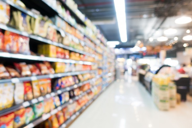
For analysis, I took pictures from the freepik.com photo stock.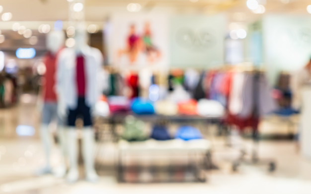
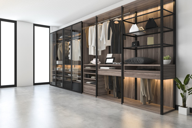
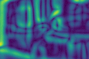
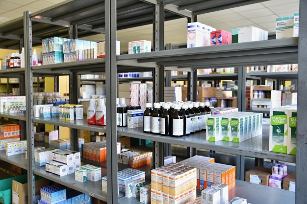 We determine the boundaries of the first picture before and after blurring:
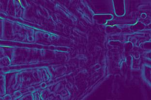
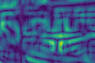
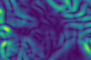 Second:
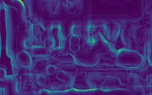
 Third:
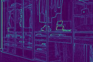
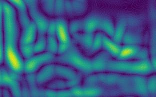
 Fourth:
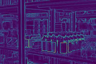
 The images show that the change in the borders of clear pictures (3rd and 4th) is stronger than that of fuzzy (1st and 2nd).After the calculations, we obtain the coefficients:[5.92918651681958,2.672756123184502,10.695051017699232,11.901115749698139]The coefficients confirm the conclusions: the larger the coefficient, the sharper the photo.Moreover, the second picture is less clear than the first, which is reflected in the coefficients.
Approach features
- the sharper the picture, the stronger the border changes, which means the higher the parameter;
- for different needs, different clarity is needed. Therefore, it is necessary to determine the boundaries of clarity on your own: somewhere, the coefficient of sufficient clear photos will be above 7, somewhere only above 10;
- the coefficient depends on the brightness of the photo. The borders of dark photos will change weaker, which means that the coefficient will be less. It turns out that the boundaries of clarity must be determined taking into account the lighting, that is, for standard photographs;
A working algorithm can be found on my github account .