Remote mode of operation against the background of universal self-isolation can lead to very bad consequences. And emotional burnout - it’s still wherever it goes: after all, it’s not far from the roof. In this regard, like many, he tried to "calm" himself by allocating time for other classes - and began to translate the most interesting articles from English into Russian: "You give machine-learning to the masses!".) We must pay tribute: it is great distracting. If you have suggestions for both semantic content and translation of this text for a Russian-speaking reader, join the discussion. So, here's a translation of the Time series forecasting page from the tensorflow manual section: link . My additions along with illustrations for the translation are aimed at helping to understand the basic ideas in one of the most interesting areas of ML and econometrics in general - forecasting time series.A small introduction before the translation.The manual is a description of air temperature prediction based on one-dimensional time series (univariate time-series) and multivariate time series (multivariate time-series) . For each part, input datashould be prepared accordingly. Taking into account the meteorological data set considered in this guide, the separation is as follows:
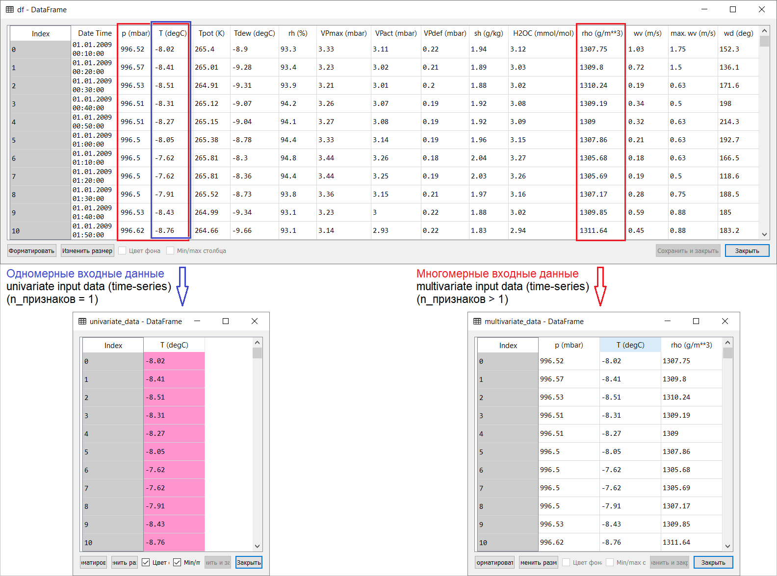 For questions about what to take for X and what for Y , that is, how to prepare data for the class of supervised training, it will become clear from the following illustrations. I only note that the formation of the target vector (Y) for working with both one-dimensional and multi-dimensional time series is the same: the target vector is compiled on the basis of the sign T (degC)(air temperature). The difference between them is “buried” in the formation of a set of features that are fed to the model’s input: in the case of a one-dimensional time series for predicting the temperature in the future, the input vector (X) consists of one feature: in fact, air temperature; and for multidimensional - more than one: in addition to air temperature, p (mbar) (atmospheric pressure) and rho (g / m ** 3) (humidity) are used in the example of the manual in question .At first, a far-shallow, look, an example with temperature forecasting looks unconvincing from the point of view of applying a multidimensional input: for temperature forecasting, the most relevant sign will be temperature. However, this is absolutely not the case: in order to develop a qualitative forecast of air temperature, many factors must be taken into account, up to air friction on the earth's surface, etc. In addition, in practice, some things are far from obvious, and the target vector may be in the form of that hodgepodge (or borsch). In this regard, exploratory data analysis with the selection of the most relevant features for the subsequent formation of a multidimensional input is the only right decision.So, the translation of the manual is presented below. Additional text will be in italics .
Time Series Forecasting
This guide is an introduction to time series forecasting using recurrent neural networks (RNS, from the English Recurrent Neural Network, RNN ). It consists of two parts: the first describes the prediction of air temperature based on a one-dimensional time series, and the second - based on a multidimensional time series.import tensorflow as tf
import matplotlib as mpl
import matplotlib.pyplot as plt
import numpy as np
import os
import pandas as pd
mpl.rcParams['figure.figsize'] = (8, 6)
mpl.rcParams['axes.grid'] = False
A set of meteorological dataAll examples of the manual use time sequences of weather data recorded at a hydrometeorological station at the Institute of Biogeochemistry named after Max Planck .This data set includes measurements of 14 different meteorological indicators (such as air temperature, atmospheric pressure, humidity), carried out every 10 minutes since 2003. To save time and memory usage, the manual will use data covering the period from 2009 to 2016. This section of the dataset was prepared by François Chollet for his book, Deep Learning with Python .zip_path = tf.keras.utils.get_file(
origin='https://storage.googleapis.com/tensorflow/tf-keras-datasets/jena_climate_2009_2016.csv.zip',
fname='jena_climate_2009_2016.csv.zip',
extract=True)
csv_path, _ = os.path.splitext(zip_path)
df = pd.read_csv(csv_path)
Let's see what we have.df.head()
 The fact that the observation recording period is 10 minutes can be verified by the table above. Thus, in one hour you will have 6 observations. In turn, 144 (6x24) observations are accumulated per day.Let's say you want to predict the temperature, which will be in 6 hours in the future. You make this forecast based on the data you have for a certain period: for example, you decide to use 5 days of observation. Therefore, to train the model, you must create a time interval containing the last 720 (5x144) observations (since different configurations are possible, this data set is a good basis for experiments).The function below returns the above time intervals for training the model. Argument
history_size- this is the size of the last time interval, target_size- an argument that determines how far into the future the model should learn to predict. In other words, target_sizeis the target vector that needs to be predicted.def univariate_data(dataset, start_index, end_index, history_size, target_size):
data = []
labels = []
start_index = start_index + history_size
if end_index is None:
end_index = len(dataset) - target_size
for i in range(start_index, end_index):
indices = range(i-history_size, i)
data.append(np.reshape(dataset[indices], (history_size, 1)))
labels.append(dataset[i+target_size])
return np.array(data), np.array(labels)
In both parts of the manual, the first 300,000 rows of data will be used to train the model, the remaining ones to validate (validate) it. In this case, the amount of training data is approximately 2100 days.TRAIN_SPLIT = 300000
To ensure reproducible results, the seed function is set.tf.random.set_seed(13)
Part 1. Forecasting based on a one-dimensional time series
In the first part, you will train the model using only one attribute - temperature; the trained model will be used to predict future temperatures.To get started, we extract only the temperature from the data set.uni_data = df['T (degC)']
uni_data.index = df['Date Time']
uni_data.head()
Date Time
01.01.2009 00:10:00 -8.02
01.01.2009 00:20:00 -8.41
01.01.2009 00:30:00 -8.51
01.01.2009 00:40:00 -8.31
01.01.2009 00:50:00 -8.27
Name: T (degC), dtype: float64
And let's see how this data changes over time.uni_data.plot(subplots=True)

uni_data = uni_data.values
Before training an artificial neural network (hereinafter - ANN), an important step is data scaling. One of the common ways of performing the scaling is standardization ( standardization ), performed by subtracting the mean and dividing by the standard deviation for each characteristic. You can also use a method tf.keras.utils.normalizethat scales values to the range [0,1].Note : standardization should only be carried out using training data.uni_train_mean = uni_data[:TRAIN_SPLIT].mean()
uni_train_std = uni_data[:TRAIN_SPLIT].std()
We perform data standardization.uni_data = (uni_data-uni_train_mean)/uni_train_std
Next, we will prepare the data for the model with a one-dimensional input. The last 20 recorded observations of the temperature will be fed to the model, and the model must be trained to predict the temperature in the next time step.univariate_past_history = 20
univariate_future_target = 0
x_train_uni, y_train_uni = univariate_data(uni_data, 0, TRAIN_SPLIT,
univariate_past_history,
univariate_future_target)
x_val_uni, y_val_uni = univariate_data(uni_data, TRAIN_SPLIT, None,
univariate_past_history,
univariate_future_target)
The results of applying the function univariate_data.print ('Single window of past history')
print (x_train_uni[0])
print ('\n Target temperature to predict')
print (y_train_uni[0])
Single window of past history
[[-1.99766294]
[-2.04281897]
[-2.05439744]
[-2.0312405 ]
[-2.02660912]
[-2.00113649]
[-1.95134907]
[-1.95134907]
[-1.98492663]
[-2.04513467]
[-2.08334362]
[-2.09723778]
[-2.09376424]
[-2.09144854]
[-2.07176515]
[-2.07176515]
[-2.07639653]
[-2.08913285]
[-2.09260639]
[-2.10418486]]

Target temperature to predict
-2.1041848598100876
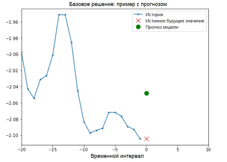
Addition: preparation of data for a model with a one-dimensional input is schematically shown in the following figure (for convenience, in this and subsequent figures, the data is presented in a raw form, before standardization, and also without the 'Date time' attribute as an index): Now that the data suitably prepared, consider a concrete example. The information transmitted to the ANN is highlighted in blue, a red cross indicates the future value that the ANN should predict.
def create_time_steps(length):
  return list(range(-length, 0))
def show_plot(plot_data, delta, title):
  labels = ['History', 'True Future', 'Model Prediction']
  marker = ['.-', 'rx', 'go']
  time_steps = create_time_steps(plot_data[0].shape[0])
  if delta:
    future = delta
  else:
    future = 0

  plt.title(title)
  for i, x in enumerate(plot_data):
    if i:
      plt.plot(future, plot_data[i], marker[i], markersize=10,
               label=labels[i])
    else:
      plt.plot(time_steps, plot_data[i].flatten(), marker[i], label=labels[i])
  plt.legend()
  plt.xlim([time_steps[0], (future+5)*2])
  plt.xlabel('Time-Step')
  return plt
show_plot([x_train_uni[0], y_train_uni[0]], 0, 'Sample Example')
 Basic solution (without involving machine learning)Before starting the model training, we will install a simple basic solution ( baseline ). It consists in the following: for a given input vector, the basic solution method “scans” the entire history and predicts the next value as the average of the last 20 observations.
def baseline(history):
  return np.mean(history)
show_plot([x_train_uni[0], y_train_uni[0], baseline(x_train_uni[0])], 0,
           'Baseline Prediction Example')
 Let's see if we can surpass the result of “averaging” using a recurrent neural network.Recurrent Neural Network Arecurrent neural network (RNS) is a type of ANN that is well suited for solving time series problems. RNS step by step processes the time sequence of data, sorting through its elements and preserving the internal state obtained by processing the previous elements. You can find more information about RNS in the following guide . This guide will use a specialized layer of RNC called Long Short-Term Memory ( LSTM ).Further using
tf.dataShuffle, batch, and cache the data set.Addition:
More about the shuffle, batch and cache methods on the tensorflow page :BATCH_SIZE = 256
BUFFER_SIZE = 10000
train_univariate = tf.data.Dataset.from_tensor_slices((x_train_uni, y_train_uni))
train_univariate = train_univariate.cache().shuffle(BUFFER_SIZE).batch(BATCH_SIZE).repeat()
val_univariate = tf.data.Dataset.from_tensor_slices((x_val_uni, y_val_uni))
val_univariate = val_univariate.batch(BATCH_SIZE).repeat()
The following visualization should help you understand what the data looks like after batch processing. It can be seen that LSTM requires a certain form of data entry, which is provided to it.
simple_lstm_model = tf.keras.models.Sequential([
    tf.keras.layers.LSTM(8, input_shape=x_train_uni.shape[-2:]),
    tf.keras.layers.Dense(1)
])

simple_lstm_model.compile(optimizer='adam', loss='mae')
Check the model output.for x, y in val_univariate.take(1):
print(simple_lstm_model.predict(x).shape)
(256, 1)
Addition:
In general terms, RNSs work with sequences. This means that the data supplied to the input of the model should have the following form:
[, , - ]
The form of training data for the model with a one-dimensional input has the following form:print(x_train_uni.shape)
(299980, 20, 1)Next, we will study the model. Due to the large size of the data set and in order to save time, each epoch will go through only 200 steps ( steps_per_epoch = 200 ) instead of the full training data, as is usually done.EVALUATION_INTERVAL = 200
EPOCHS = 10
simple_lstm_model.fit(train_univariate, epochs=EPOCHS,
steps_per_epoch=EVALUATION_INTERVAL,
validation_data=val_univariate, validation_steps=50)
Train for 200 steps, validate for 50 steps
Epoch 1/10
200/200 [==============================] - 2s 11ms/step - loss: 0.4075 - val_loss: 0.1351
Epoch 2/10
200/200 [==============================] - 1s 4ms/step - loss: 0.1118 - val_loss: 0.0360
Epoch 3/10
200/200 [==============================] - 1s 4ms/step - loss: 0.0490 - val_loss: 0.0289
Epoch 4/10
200/200 [==============================] - 1s 4ms/step - loss: 0.0444 - val_loss: 0.0257
Epoch 5/10
200/200 [==============================] - 1s 4ms/step - loss: 0.0299 - val_loss: 0.0235
Epoch 6/10
200/200 [==============================] - 1s 4ms/step - loss: 0.0317 - val_loss: 0.0224
Epoch 7/10
200/200 [==============================] - 1s 4ms/step - loss: 0.0287 - val_loss: 0.0206
Epoch 8/10
200/200 [==============================] - 1s 4ms/step - loss: 0.0263 - val_loss: 0.0200
Epoch 9/10
200/200 [==============================] - 1s 4ms/step - loss: 0.0254 - val_loss: 0.0182
Epoch 10/10
200/200 [==============================] - 1s 4ms/step - loss: 0.0228 - val_loss: 0.0174
Prediction using a simple LSTM modelAfter completing the preparation of a simple LSTM model, we will make several predictions.for x, y in val_univariate.take(3):
plot = show_plot([x[0].numpy(), y[0].numpy(),
simple_lstm_model.predict(x)[0]], 0, 'Simple LSTM model')
plot.show()
 It looks better than the base level.Now that you’ve become familiar with the basics, let's move on to the second part, which describes working with a multidimensional time series.
Part 2: Multidimensional Time Series Forecasting
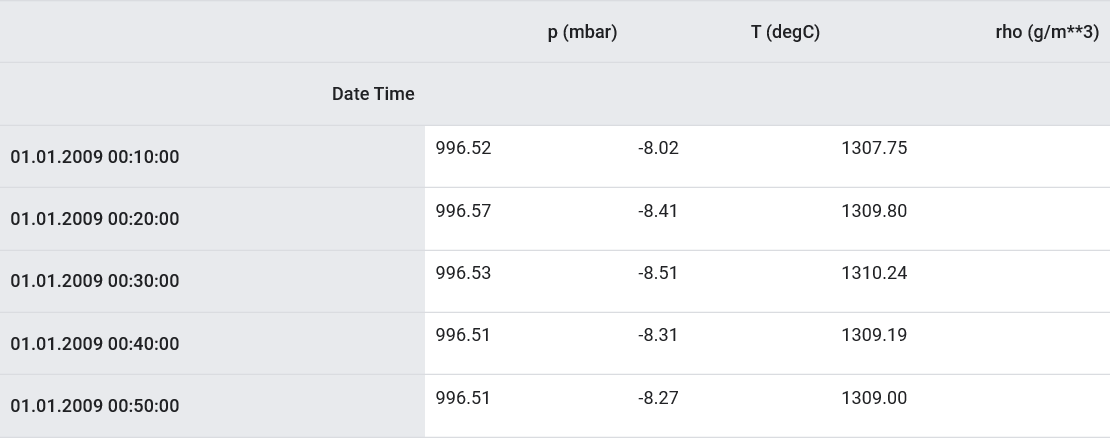
As stated, the original dataset contains 14 different meteorological indicators. For simplicity and convenience, in the second part only three of them are considered - air temperature, atmospheric pressure and air density.To use more features, their names must be added to the feature_considered list .features_considered = ['p (mbar)', 'T (degC)', 'rho (g/m**3)']
features = df[features_considered]
features.index = df['Date Time']
features.head()
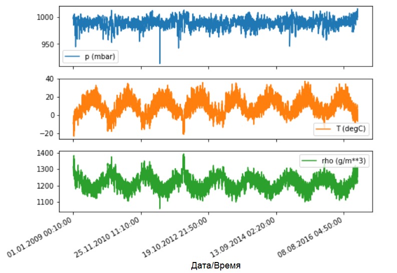
 Let's see how these indicators change over time.
features.plot(subplots=True)
 As before, the first step is to standardize the data set with the calculation of the average value and standard deviation of the training data.
dataset = features.values
data_mean = dataset[:TRAIN_SPLIT].mean(axis=0)
data_std = dataset[:TRAIN_SPLIT].std(axis=0)
dataset = (dataset-data_mean)/data_std
Addition:
Further in the manual we will talk about point and interval forecasting.
The bottom line is as follows. If you need the model to predict one value in the future (for example, the temperature value after 12 hours) (one-step / single step model), then you must train the model so that it predicts only one value in the future. If the task is to predict the range of values in the future (for example, hourly temperatures over the next 12 hours) (multi-step model), then the model should also be trained to predict the range of values in the future. Point predictionIn this case, the model is trained to predict one value in the future based on some available history.The function below performs the same task of organizing time intervals only with the difference that here it selects the latest observations based on a given step size.
def multivariate_data(dataset, target, start_index, end_index, history_size,
                      target_size, step, single_step=False):
  data = []
  labels = []

  start_index = start_index + history_size
  if end_index is None:
    end_index = len(dataset) - target_size

  for i in range(start_index, end_index):
    indices = range(i-history_size, i, step)
    data.append(dataset[indices])

    if single_step:
      labels.append(target[i+target_size])
    else:
      labels.append(target[i:i+target_size])

  return np.array(data), np.array(labels)
In this guide, the ANN operates on data for the last five (5) days, i.e. 720 observations (6x24x5). Suppose that the selection of data is carried out not every 10 minutes, but every hour: within 60 minutes, sharp changes are not expected. Therefore, the history of the last five days consists of 120 observations (720/6). For a model that performs spot prediction, the goal is to read the temperature after 12 hours in the future. In this case, the target vector will be the temperature after 72 (12x6) observations ( see the following addition. - Approx. Translator ).past_history = 720
future_target = 72
STEP = 6
x_train_single, y_train_single = multivariate_data(dataset, dataset[:, 1], 0,
TRAIN_SPLIT, past_history,
future_target, STEP,
single_step=True)
x_val_single, y_val_single = multivariate_data(dataset, dataset[:, 1],
TRAIN_SPLIT, None, past_history,
future_target, STEP,
single_step=True)
Check the time interval.print ('Single window of past history : {}'.format(x_train_single[0].shape))
Single window of past history : (120, 3)
train_data_single = tf.data.Dataset.from_tensor_slices((x_train_single, y_train_single))
train_data_single = train_data_single.cache().shuffle(BUFFER_SIZE).batch(BATCH_SIZE).repeat()

val_data_single = tf.data.Dataset.from_tensor_slices((x_val_single, y_val_single))
val_data_single = val_data_single.batch(BATCH_SIZE).repeat()
single_step_model = tf.keras.models.Sequential()
single_step_model.add(tf.keras.layers.LSTM(32,
                                           input_shape=x_train_single.shape[-2:]))
single_step_model.add(tf.keras.layers.Dense(1))

single_step_model.compile(optimizer=tf.keras.optimizers.RMSprop(), loss='mae')
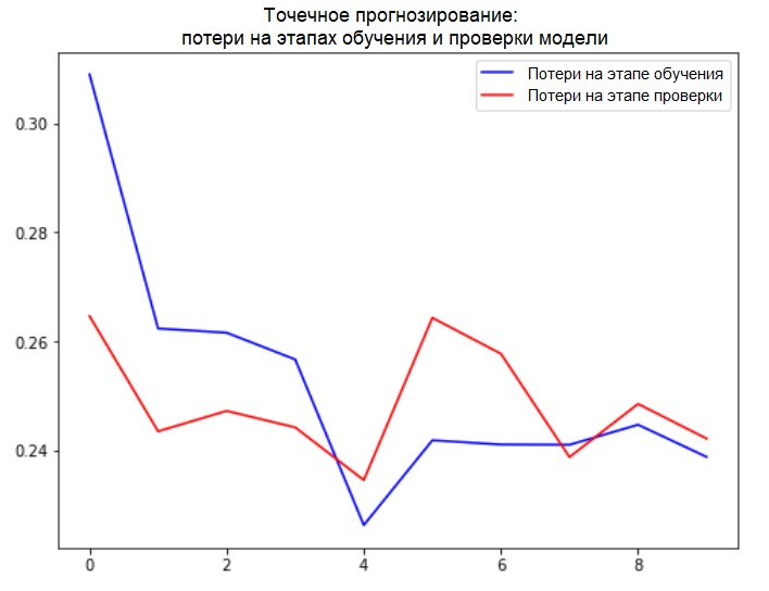
We will check our sample and derive loss curves at the stages of training and verification.for x, y in val_data_single.take(1):
print(single_step_model.predict(x).shape)
(256, 1)
single_step_history = single_step_model.fit(train_data_single, epochs=EPOCHS,
                                            steps_per_epoch=EVALUATION_INTERVAL,
                                            validation_data=val_data_single,
                                            validation_steps=50)
Train for 200 steps, validate for 50 steps
Epoch 1/10
200/200 [==============================] - 4s 18ms/step - loss: 0.3090 - val_loss: 0.2646
Epoch 2/10
200/200 [==============================] - 2s 9ms/step - loss: 0.2624 - val_loss: 0.2435
Epoch 3/10
200/200 [==============================] - 2s 9ms/step - loss: 0.2616 - val_loss: 0.2472
Epoch 4/10
200/200 [==============================] - 2s 9ms/step - loss: 0.2567 - val_loss: 0.2442
Epoch 5/10
200/200 [==============================] - 2s 9ms/step - loss: 0.2263 - val_loss: 0.2346
Epoch 6/10
200/200 [==============================] - 2s 9ms/step - loss: 0.2416 - val_loss: 0.2643
Epoch 7/10
200/200 [==============================] - 2s 9ms/step - loss: 0.2411 - val_loss: 0.2577
Epoch 8/10
200/200 [==============================] - 2s 9ms/step - loss: 0.2410 - val_loss: 0.2388
Epoch 9/10
200/200 [==============================] - 2s 9ms/step - loss: 0.2447 - val_loss: 0.2485
Epoch 10/10
200/200 [==============================] - 2s 9ms/step - loss: 0.2388 - val_loss: 0.2422
def plot_train_history(history, title):
  loss = history.history['loss']
  val_loss = history.history['val_loss']

  epochs = range(len(loss))

  plt.figure()

  plt.plot(epochs, loss, 'b', label='Training loss')
  plt.plot(epochs, val_loss, 'r', label='Validation loss')
  plt.title(title)
  plt.legend()

  plt.show()
plot_train_history(single_step_history,
                   'Single Step Training and validation loss')
 Addition:
Data preparation for a model with a multidimensional input performing point prediction is shown schematically in the following figure. For convenience and a more visual representation of data preparation, the argument STEPis 1. Note that in the given generator functions, the argument is STEP intended only for the formation of the history , and not for the target vector.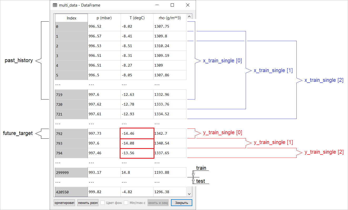 In this case, it
 x_train_singlehas the form (299280, 720, 3).
When STEP=6, the form will take the following form: (299280, 120, 3)and the speed of the function will increase significantly. In general, you need to give credit to the programmer: the generators presented in the manual are very voracious in terms of memory consumption.Performing a point predictionNow that the model is trained, we will perform several test predictions. The history of observations of 3 signs for the last five days, selected every hour (time interval = 120), is fed to the model input. Since our goal is to forecast only temperature, the past temperature values ( history ) are displayed in blue on the graph . The forecast was made half a day into the future (hence the gap between history and the predicted value).for x, y in val_data_single.take(3):
plot = show_plot([x[0][:, 1].numpy(), y[0].numpy(),
single_step_model.predict(x)[0]], 12,
'Single Step Prediction')
plot.show()
 Interval forecastingIn this case, on the basis of some available history, the model is trained to predict the interval of future values. Thus, in contrast to a model that predicts only one value in the future, this model predicts a sequence of values in the future.Suppose, as in the case with the model performing point prediction, for the model performing interval prediction, the training data is the hourly measurements of the last five days (720/6). However, in this case, the model must be trained to predict the temperature for the next 12 hours. Since observations are recorded every 10 minutes, the output of the model should consist of 72 predictions. To complete this task, it is necessary to prepare the data set again, but with a different target interval.
future_target = 72
x_train_multi, y_train_multi = multivariate_data(dataset, dataset[:, 1], 0,
                                                 TRAIN_SPLIT, past_history,
                                                 future_target, STEP)
x_val_multi, y_val_multi = multivariate_data(dataset, dataset[:, 1],
                                             TRAIN_SPLIT, None, past_history,
                                             future_target, STEP)
Check the selection.print ('Single window of past history : {}'.format(x_train_multi[0].shape))
print ('\n Target temperature to predict : {}'.format(y_train_multi[0].shape))
Single window of past history : (120, 3)

Target temperature to predict : (72,)
train_data_multi = tf.data.Dataset.from_tensor_slices((x_train_multi, y_train_multi))
train_data_multi = train_data_multi.cache().shuffle(BUFFER_SIZE).batch(BATCH_SIZE).repeat()

val_data_multi = tf.data.Dataset.from_tensor_slices((x_val_multi, y_val_multi))
val_data_multi = val_data_multi.batch(BATCH_SIZE).repeat()
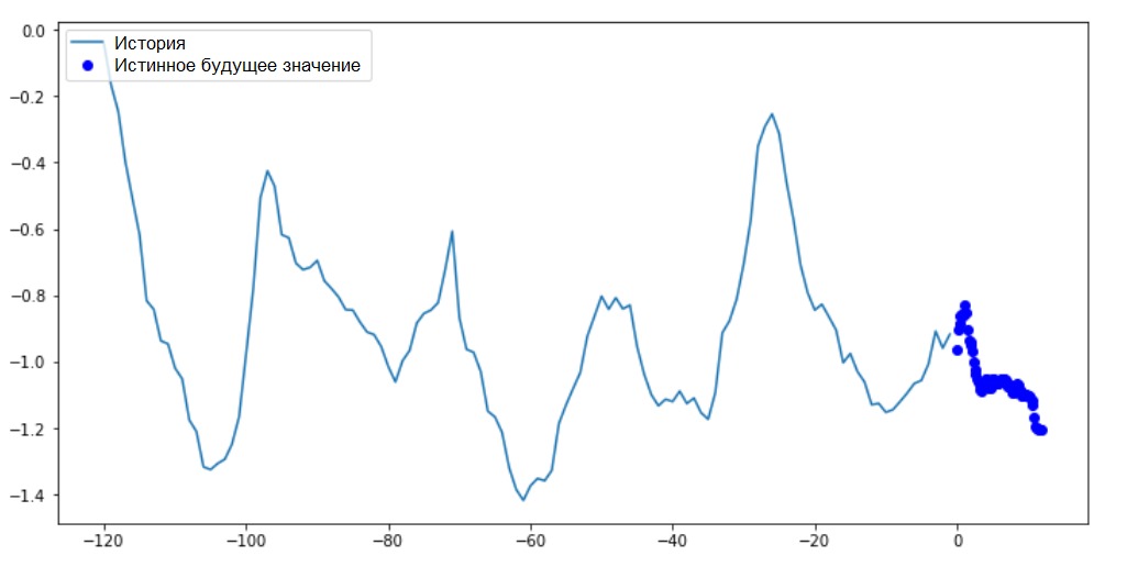
Addition: the difference in the formation of the target vector for the “interval model” from the “point model” is seen in the following figure. We will prepare the visualization.
def multi_step_plot(history, true_future, prediction):
  plt.figure(figsize=(12, 6))
  num_in = create_time_steps(len(history))
  num_out = len(true_future)

  plt.plot(num_in, np.array(history[:, 1]), label='History')
  plt.plot(np.arange(num_out)/STEP, np.array(true_future), 'bo',
           label='True Future')
  if prediction.any():
    plt.plot(np.arange(num_out)/STEP, np.array(prediction), 'ro',
             label='Predicted Future')
  plt.legend(loc='upper left')
  plt.show()
On this and subsequent similar charts, the history and future data are hourly.for x, y in train_data_multi.take(1):
multi_step_plot(x[0], y[0], np.array([0]))
 Since this task is a bit more complicated than the previous one, the model will consist of two LSTM layers. Finally, since 72 predictions are performed, the output layer has 72 neurons.
multi_step_model = tf.keras.models.Sequential()
multi_step_model.add(tf.keras.layers.LSTM(32,
                                          return_sequences=True,
                                          input_shape=x_train_multi.shape[-2:]))
multi_step_model.add(tf.keras.layers.LSTM(16, activation='relu'))
multi_step_model.add(tf.keras.layers.Dense(72))

multi_step_model.compile(optimizer=tf.keras.optimizers.RMSprop(clipvalue=1.0), loss='mae')
We will check our sample and derive loss curves at the stages of training and verification.for x, y in val_data_multi.take(1):
print (multi_step_model.predict(x).shape)
(256, 72)
multi_step_history = multi_step_model.fit(train_data_multi, epochs=EPOCHS,
                                          steps_per_epoch=EVALUATION_INTERVAL,
                                          validation_data=val_data_multi,
                                          validation_steps=50)
Train for 200 steps, validate for 50 steps
Epoch 1/10
200/200 [==============================] - 21s 103ms/step - loss: 0.4952 - val_loss: 0.3008
Epoch 2/10
200/200 [==============================] - 18s 89ms/step - loss: 0.3474 - val_loss: 0.2898
Epoch 3/10
200/200 [==============================] - 18s 89ms/step - loss: 0.3325 - val_loss: 0.2541
Epoch 4/10
200/200 [==============================] - 18s 89ms/step - loss: 0.2425 - val_loss: 0.2066
Epoch 5/10
200/200 [==============================] - 18s 89ms/step - loss: 0.1963 - val_loss: 0.1995
Epoch 6/10
200/200 [==============================] - 18s 90ms/step - loss: 0.2056 - val_loss: 0.2119
Epoch 7/10
200/200 [==============================] - 18s 91ms/step - loss: 0.1978 - val_loss: 0.2079
Epoch 8/10
200/200 [==============================] - 18s 89ms/step - loss: 0.1957 - val_loss: 0.2033
Epoch 9/10
200/200 [==============================] - 18s 90ms/step - loss: 0.1977 - val_loss: 0.1860
Epoch 10/10
200/200 [==============================] - 18s 88ms/step - loss: 0.1904 - val_loss: 0.1863
plot_train_history(multi_step_history, 'Multi-Step Training and validation loss')
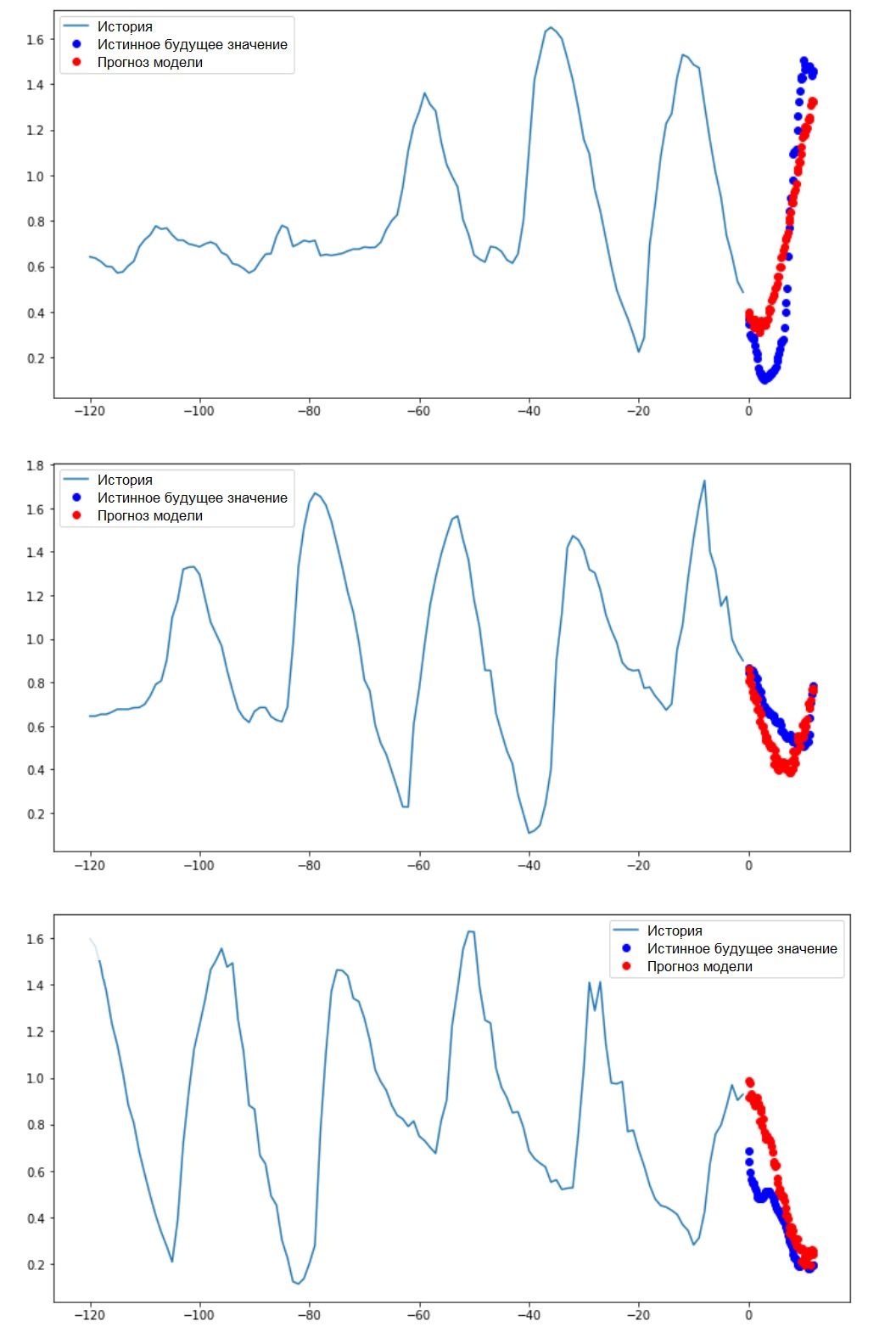
 Performing an Interval PredictionSo, let's find out how successfully a trained ANN copes with forecasts of future temperature values.
for x, y in val_data_multi.take(3):
  multi_step_plot(x[0], y[0], multi_step_model.predict(x)[0])
Next steps
This guide is a brief introduction to time series forecasting using RNS. Now you can try to predict the stock market and become a billionaire (in the original, just like that :). - Note translator) .In addition, you can write your own generator for preparing data instead of the uni / multivariate_data function in order to make more efficient use of memory. You can also familiarize yourself with the work of “ time series windowing ” and bring its ideas to this guide.For further understanding, it is recommended that you read Chapter 15 of the book “Applied Machine Learning with Scikit-Learn, Keras, and TensorFlow” (Aurelien Geron, 2nd Edition) and Chapter 6 of the book“Deep Learning in Python” (Francois Scholl).Final addition
While staying at home, take care not only about your health, but also take pity on the computer by executing examples of the manual on a truncated data set. For example, taking into account the proportion of 70x30 (training / testing), you can limit it as follows:dataset = features[300000:].values
TRAIN_SPLIT = 85000