 The SDR receiver, even the cheapest, is a highly sensitive instrument. If you add a special antenna and OpenCV to it, you can not only habitually listen to the ether, but also look at the distribution of electromagnetic fields in space. Such an interesting application will be discussed in this article. Attention! Under the cut a lot of pictures and animations!Would you like to see electromagnetic fields? Yes, there is nothing easier, here they are:
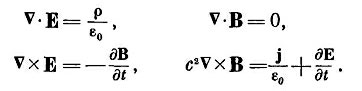 I agree, not very clearly. Even if we are able to see light (which is also described by these equations), then the radio spectrum is not so easily accessible for us. For this reason, mankind has come up with many different ways to spy on this mystery of nature, using both computer modeling and specialized installations.The latter can be found within the walls of scientific institutes, research departments of large companies and, of course, the military. Usually this is a separate room, shielded from external radiation by a Faraday cage, and from the inside covered with radar absorbing materials. After all, a neighbor-amateur or an ungrounded microwave should not bother us when conducting such experiments. This room is called anechoic chamber. The name is of course more consistent with the recording studio, but in this case, “echo” refers to any internal reflections and re-reflections of electromagnetic waves that interfere with research and are mercilessly quenched. Inside the camera, from the point of view of the antenna, you are in an absolute void, where all the radiation goes into endless expanses simulated by a radio absorber and nothing comes back.
, -, , - — , , . «»
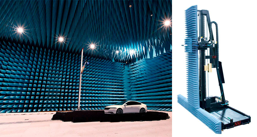 , Panasonic. « » — . — .When conducting tests for electromagnetic compatibility, the development of antennas, as well as scientific research related to electromagnetic radiation, one cannot do without such cameras. However, the camera itself is only part of the story. Among other key elements necessary to record the behavior of electromagnetic waves, special antennas, expensive measuring instruments, and, in fact, a field scanner will also be needed. The scanner is nothing more than the notorious coordinate system with CNC. You can give the scanner a suitable antenna or a measuring probe in your “hand”, and then go to drink coffee until it carefully walks around the points set by the program, constructing a beautiful picture of the distribution of fields around your new tank or, for example, the radiation pattern of the radar.But back to the point. It just so happened that far from sources, in empty space, electromagnetic fields look pretty boring. Something like this:
 While the most magic and interesting things lurk in regions where waves form (near sources), or interact with objects. These areas usually do not exceed the dimensions of the wavelength of radio emission, which is involved in the experiment, and are called the near-field zone. Investigations of the near field fields are undoubtedly one of the most curious, and of course they could not stay long only behind the shielded walls of large organizations.Enthusiasts quickly realized that for mapping fields on the same principle as in professional cameras, you can build your own coordinate scanner, or, even simpler, adapt the ubiquitous 3d printers for this purpose. Why, really, they even wrote a scientific article about it.
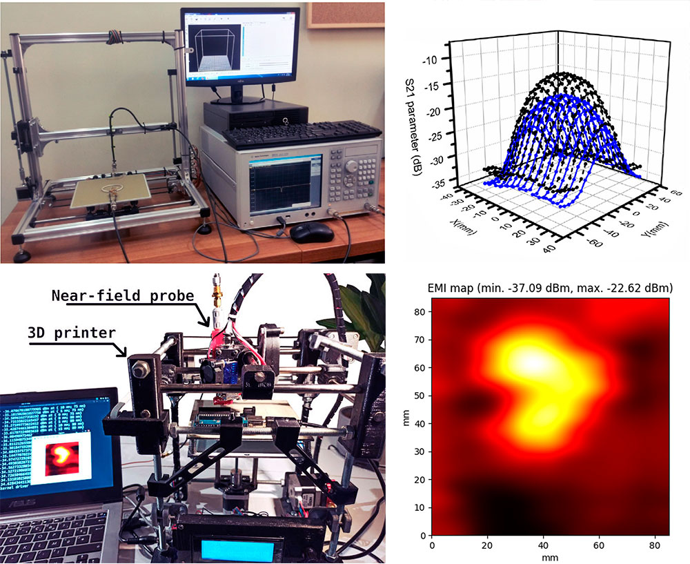 3d-printers, where instead of the extruder (or with it) are installed measuring probes, antennas. It is shown above how the coupling coefficient of two loop antennas: the measuring one, and the one lying on the printer table (the so-called S21 parameter) changes in space. Below is an example of constructing the distribution of a high-frequency magnetic field over an Arduino shawl.Although homemade scanners are not in the electromagnetically sterile environment of anechoic chambers, they can still produce interesting results. And if in the first example from the picture above an expensive professional analyzer is used to collect data (a scientific article, after all), then in the second case they cost an inexpensive SDR receiver, which makes such experiments even more affordable. However, we will not dwell on 3d printers, they are already tired of everything in order.The author of the second project from the picture, Charles Grassin , decided to simplify the process even more, and completely get rid of any coordinate system, like an extra bulky element, offering to track the movement of the measuring antenna using OpenCV. The system he conceived looks like this:
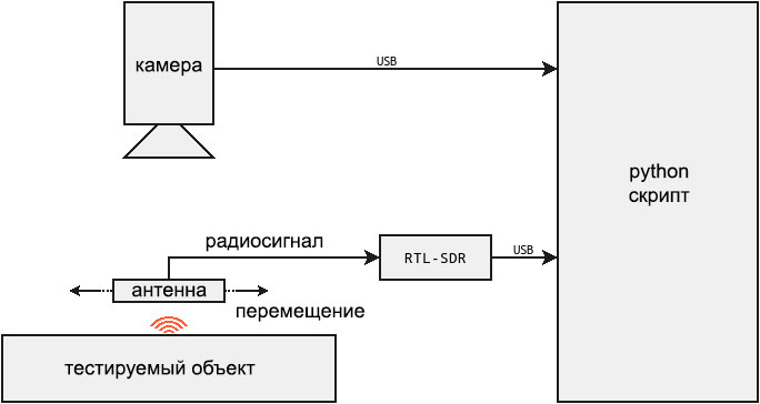 Installation diagram for mapping electromagnetic fields using an SDR receiver and OpenCV.A camera is installed above the object whose field we want to see. The script sets how our antenna looks, and then we draw it, just like a brush, in the areas where we want to see the field. The signal from the antenna goes to the SDR receiver and the python script compares the position of the antenna in the frame with the rms signal level from the receiver. After which we get a beautiful picture with the distribution of fields. Of course, this approach so far limits us to one plane, but this does not make it less interesting. Let's build this system and check how it works, since a lot of details are not required for this.First we decide what exactly we will measure. Despite the fact that electromagnetic fields are a single phenomenon, we can separately look at both its electric and magnetic components. Each type will require its own special measuring antenna. Like the author of the original, I made a probe antenna for a magnetic field according to the scheme below:
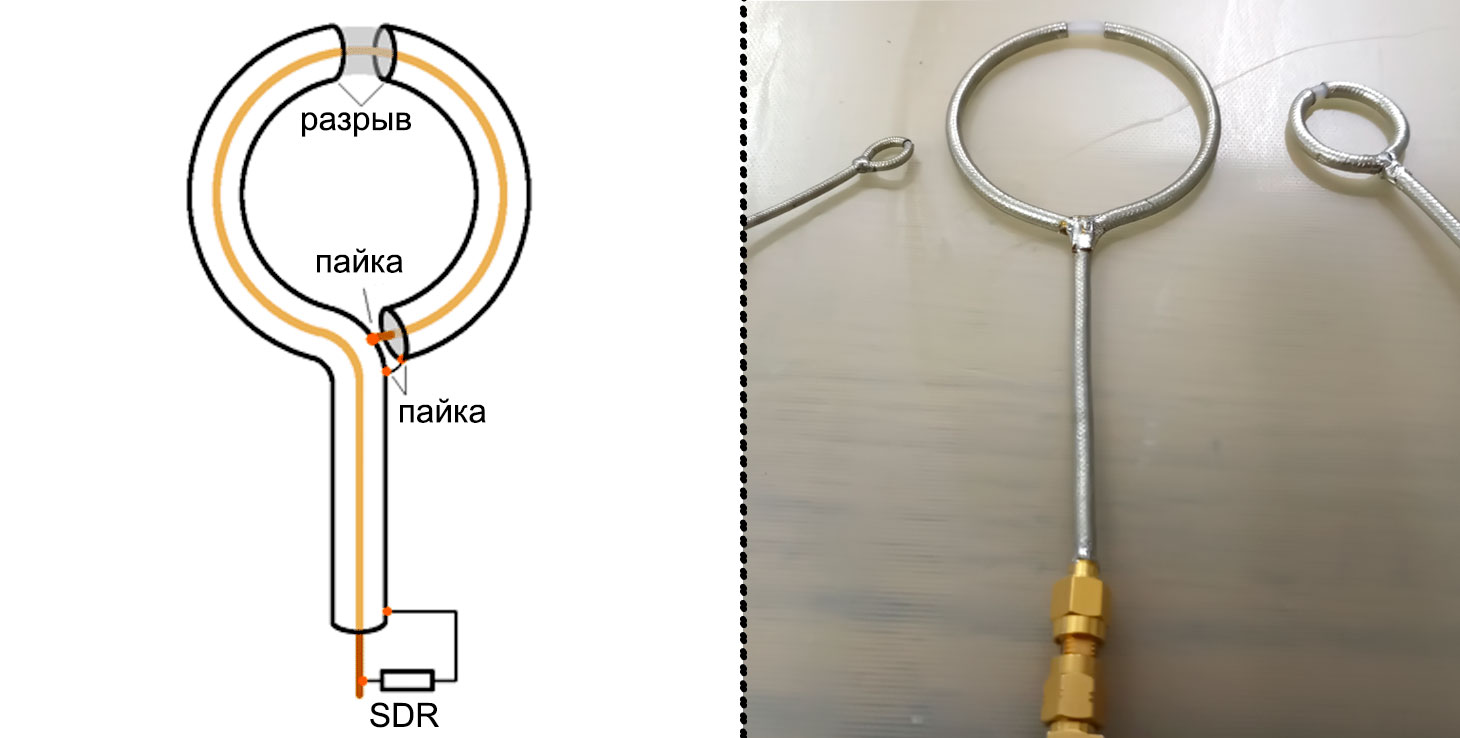 A scheme for manufacturing a magnetic probe and examples that I made. If you took the mapping of fields seriously, then make a lot of antennas of different sizes - come in handy. Even if it doesn’t come out with margins, then there will be a good set for blowing soap bubbles.This design is well known to hams under the name of a loop antenna, however, unlike older brothers, this antenna does not have to be coordinated with the receiver, which certainly simplifies our life. As a basis for a probe, it is best to use a hard or semi-hard coaxial cable, but in principle, you can do almost anything. Cable impedance also does not play a role. What is important is the size of the antenna, as we will see later.To demonstrate how the probe “feels” the different components of the electromagnetic field, I modeled it in CST:
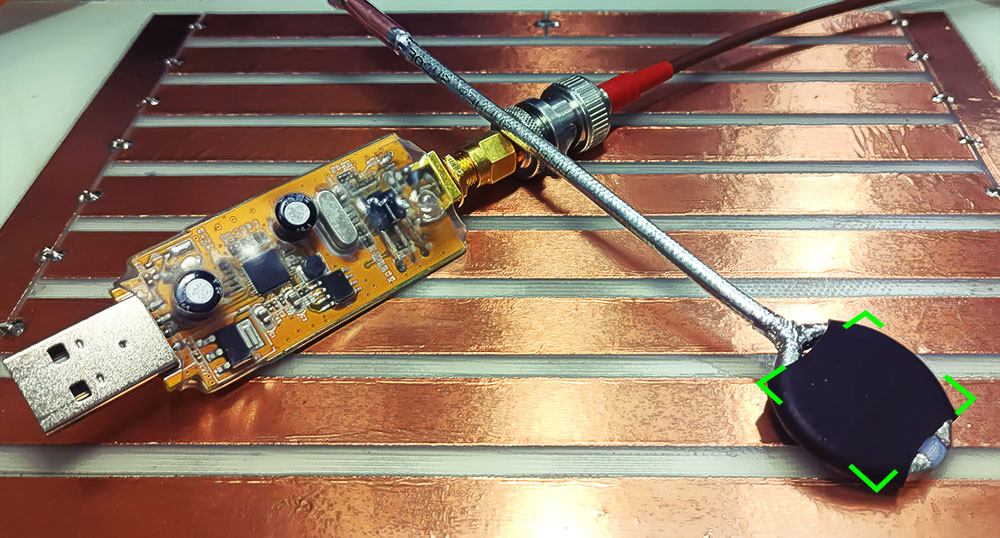
 , , . — , ( ). . .Even as two manifestations of a single entity, the electric and magnetic fields interact with the antenna in different ways. The gap in the braid that we made from above is nothing but an air condenser. As befits a capacitor, it concentrates the electric field in its gap. The magnetic field, due to the symmetry of the structure, has a maximum inside the loop. Thus, if we want to measure the latter, it is enough to place the loop parallel to the measured object. And this is just what you need to capture it in the frame using OpenCV! So, after the antenna is ready, add the final touch. We will improve its visual recognition by using black heat shrink or electrical tape. Here is my work:
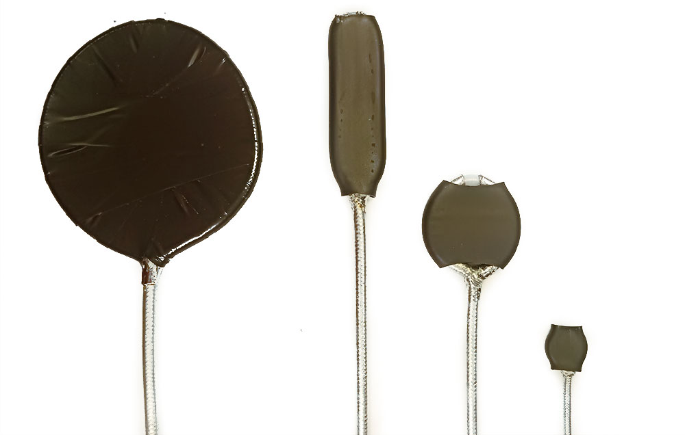 For the largest antenna (5 cm in diameter), there was no shrinkage of the required size. However, in the end I did not use it. Black will give a great contrast to the white background so that OpenCV makes it easier to see our antenna.Next, you need to get a webcam and install it on a kind of tripod. If suddenly you did not have a webcam, then a smartphone on android with the DroidCam application is also suitable. The antenna is connected to the SDR receiver, and he, in turn, to the computer. The hardware is ready for this.Download the camera_emi_mapper.py script . It will require the opencv and pyrtlsdr libraries to work.. Detailed installation instructions are available at the designated link. Please note that if you use Windows, then the pyrtlsdr libraries should be of the same bit depth as the python version on your system. The script is launched by the command:
python3 camera_emi_mapper.py -c 1 -f 100
the -c flag allows you to select a camera if you have several of them, and the -f flag sets the frequency at which the signal magnitude will be monitored (in megahertz). If everything works, then we will see the image from the webcam. For the first test experiment, I placed my OSA103 device in the frame , turning it on in the generator mode at 100 MHz : We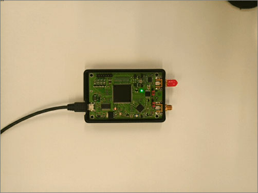 press R so that the script remembers the background image, and then we put a loop into the scanning zone. Then, using the S key, you can select our antenna in the following way:
 After confirming your choice with the Enter key, data capture from the camera and the SDR receiver will immediately begin. Well, and as usual, the first time everything goes wrong:
 To understand what OpenCV sees and why the capture does not work as it should, I uncommented the following lines of the script:
They open two additional windows where you can see how well the antenna contrasts with the background image. This contrast is adjusted by the value in thresh :
thresh = cv2.threshold(frameDelta, 50, 255, cv2.THRESH_BINARY)[1]
In the original it was 15, I increased this value to 50, and the antenna began to be confidently captured. This number must be selected depending on the lighting in the frame. At the same time, I experimented with the brightness of the antenna, since black sometimes got confused with a large square FPGA. After these corrections, everything began to work like a clock: When the scan is completed, you need to press Q and the script will build the field distribution. In this case, the result is as follows:
 Honestly - little is understood, everything turned out to be blurry and with some kind of divorce. Not that I was expecting a super result, but I would like to see something more specific, for example, which circuits in the device are involved in the generation. Still, the mapping of electromagnetic fields should give answers to questions and not create new ones. I looked again at the code and saw that the picture of the field was very blurry during construction. I reduced this effect by changing the sigma value from 7 to 2:
blurred = gaussian_with_nan(powermap, sigma=2)
Also, I replaced the measurement object. To test the method, you need some simpler thing as a test subject, and a device with a complex internal structure is not suitable for this. Moreover, the distribution of the radio frequency magnetic field of the new object must be known in advance so that it is clear whether the script shows the fields correctly or not. The same magnetic loop fits perfectly with this criterion. As we saw earlier, in a loop, the magnetic field is concentrated inside its loop. So, when scanning, we should see it. I soldered a simple square resonant circuit of the form of copper foil and capacitor: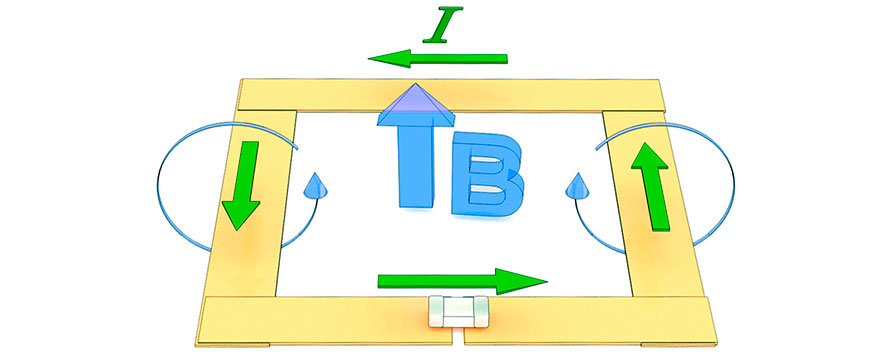 , . , . , .You may have a question - how can we see the field in this way, if there is not even any source here! And the thing is that we are surrounded by white noise (the same “noise” that we hear when we are not tuned to a favorite station), and in its spectrum there are already almost any desired frequencies. If we bring the measuring antenna close to the resonant circuit, it will become more susceptible to noise at the resonant frequency of this circuit itself. The SDR receiver is so sensitive that it can even be used to measure fields in passive objects! Let's try what happens:
 I tried to act very carefully, but still in the process I slightly shifted the sheet on which the contour was glued. However, the result was not bad. You can drive our probe much faster. As I understand it, the speed of data processing depends only on the performance of the computer and the tremor of your hands. In any case, the video card of my laptop noticeably strained during the testing process. Yes, and I also changed the color map to a more pleasant plasma for the eyes:
 It seems that the practice nevertheless coincides with the theory and the working method. We see the magnetic field where it was expected - inside the circuit. At the same time, the resolution of our image is directly dictated by the size of the measuring antenna, which is why the fields are a little out of place where they are physically. And this is the reason why the size of the antenna is so important, because the magnitude of this shift will depend on it. It is also clearly seen that a change in the direction of movement of the antenna distorts the picture. This is because the process of such "drawing" reminds me suspiciously of something:
 By analogy with the example above, the method gives good resolution in the direction of movement of the antenna. But with each change in this direction, an error creeps into the data in the form of a displacement of the field picture. I circled the same outline, but this time diagonally, which once again demonstrated this drawback. By the way, both scans were carried out at a frequency of 87 MHz.
 Unfortunately, I am a so-so programmer, because I have not yet figured out how to modify the code to fix this error. Instead, I can offer a brief authoring methodology for measuring fields. We call it a single stroke technique:
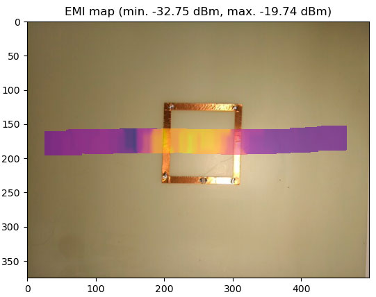 Everything is simple - if there is one direction, then there are no errors. Of course, while this limits the scope of possible applications even more, but we will be sure that the observed fields more or less correspond to reality. Now, being aware of how to measure correctly, you can try to scan something else. For example, did you know that a resonant circuit, like the one already shown, can be done without conductors at all? As I have already argued, a high-frequency current flows through a capacitor, which means that you can assemble a resonant circuit using only it and nothing more. Mentally increase the capacitor many times and get a piece of ceramic that also localizes the magnetic field near it (thanks to colleagues from ITMO for the provided sample). Scanning frequency 254 MHz.
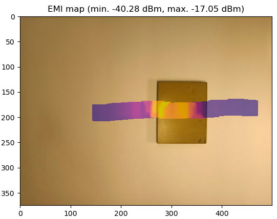 It is worth mentioning another drawback of the method - the distance from the object to the antenna should ideally be the same, otherwise our picture of the fields will no longer be in the plane, which means it will be distorted. Theoretically, I think this can also be fixed using OpenCV, by tracking the change in the size of the antenna in the frame.For the final demonstration, I put together such a more complicated thing:
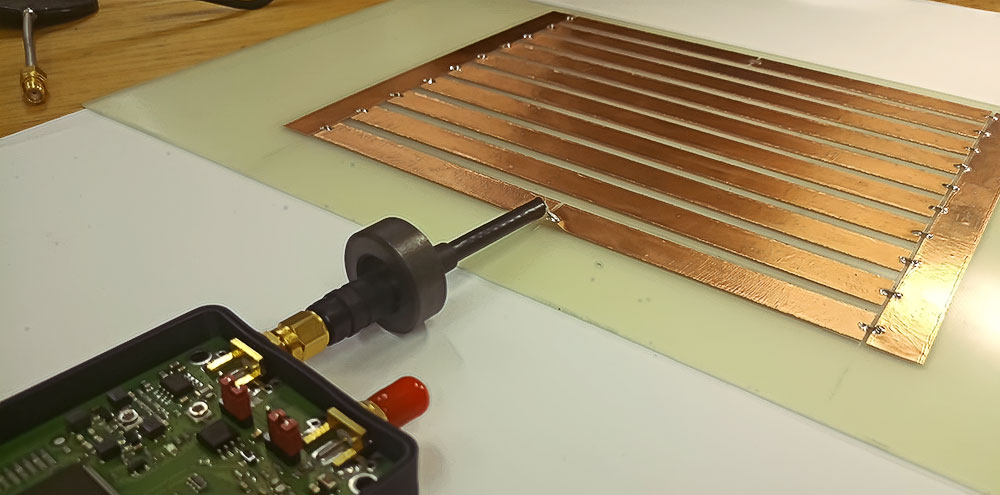 This is a multi-stage low-pass filter, it can also be called a transmission line, or even metamaterial (with a very big stretch). The circuit diagram looks like this:
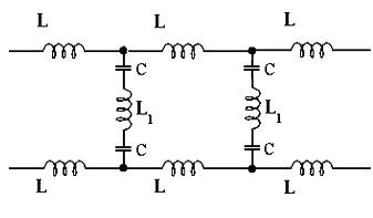 Since there are a lot of resonant elements in this structure, it also has a lot of resonant frequencies (measured by the device from the first experiment). Each minimum of the graph is a resonance in the spectrum:
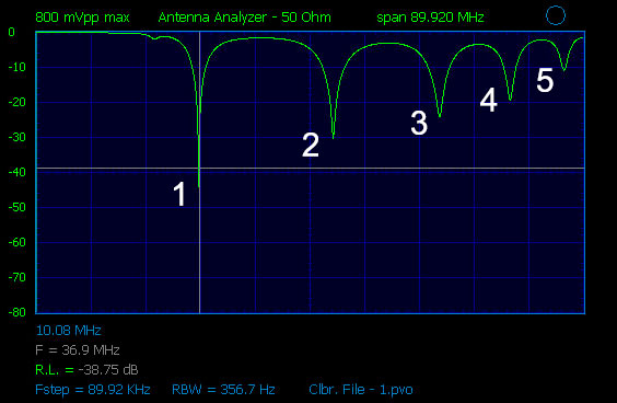 Such resonances are called eigenmodes. And each of them has its own unique picture of the fields. But nevertheless, they are all connected by a certain regularity, namely, the number of waves that fit into the structure, which is clearly visible when scanning:
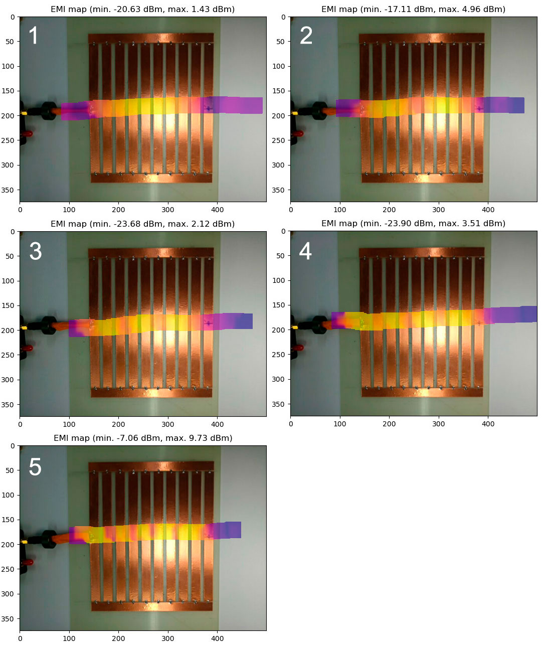 Having counted the number of field peaks, you can accurately name the mode number. It is also a great illustration of how electromagnetic fields reduce their speed inside materials. After all, the wave velocity is less - more field peaks fit in the picture. In my opinion, a great visual aid.As you can see, the idea of crossing SDR and OpenCV turned out to be quite good. And most importantly, this union brings a creative touch to the boring and monotonous measurement process. I think in the future it can make the study of electromagnetic fields a more exciting experience, as well as become a good help for home laboratories.