Coderikonce noted: "There are never too many Kalman filters . " The same can be said about Bayes's theorem, because on the one hand it is so simple, but on the other hand it is so difficult to comprehend its depth.
YouTube has a wonderful Student Dave channel , but the last video was posted six years ago. The channel contains educational videos in which the author tells complex things in a very simple language: Bayes theorem, Kalman filter, etc. Student Dave complements his story with an example of calculation in matlab.
Once his video lesson called “Iterative Bayesian Assessment” really helped me a lot (on the channel it corresponds to the playlist “Iterative bayesian estimation: with MATLAB”) I wanted everyone to get acquainted with Dave's explanations, but unfortunately the project is not supported. Dave himself does not get in touch. You can’t add a translation to the video, as the author himself must initiate it. Contacting youtube did not give a result, so I decided to describe the material in an article in Russian and publish where it is most appreciated. The material is very much revised and supplemented, as it went through my subjective perception, so putting it as a translation would be inappropriate. But I took the very salt of the explanation from Dave. I rewrote its code in python, since I myself work in it and consider it a good substitute for mathematical packages.
So, if you want to make a deeper understanding of the topic of Bayes' theorem, welcome.
Formulation of the problem
, “ ”. .
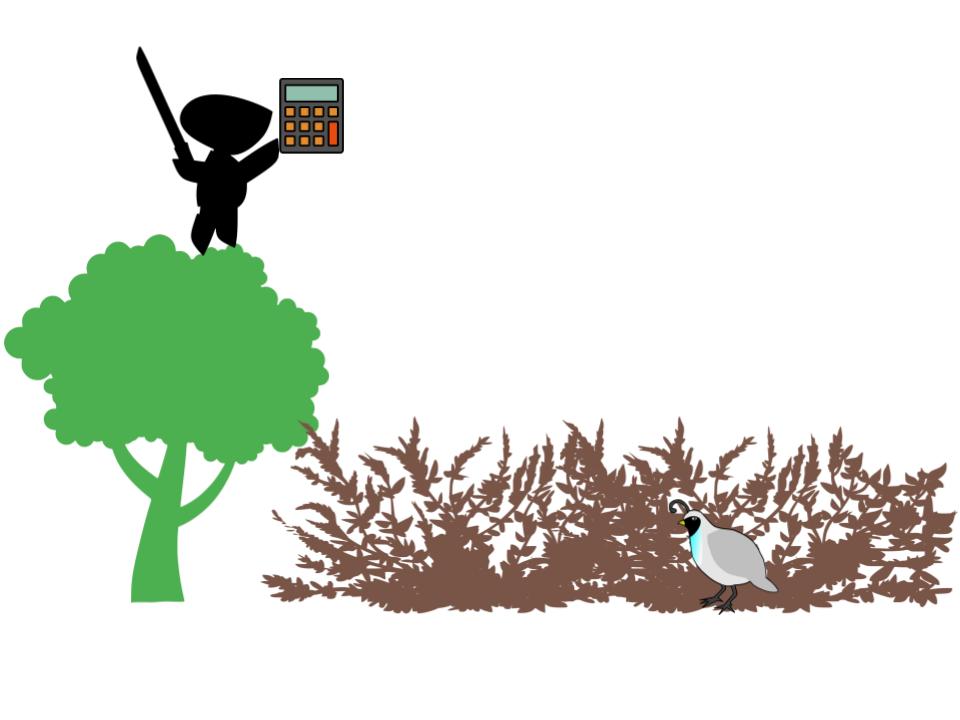
-, . , . , . . , . . - .
- . . . .

( ) () .
.
, .
— ;
— ;
— ( ).
. , ( , ):
— ;
— ;
— ;
— .
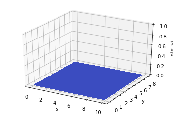
(), , .
.

.
, 99,7 %.
. -.
. ( ) .
() , . .
:
— ;
— ;
— ;
— .
:
— ;
— .
, .
.
Thus, it is seen how the results of the experiment affect the a priori distribution. If you use the measurements correctly, you can get good accuracy.
But isn’t it easier to just find the average of all measurements and thus make an assessment of the location of the quail? Of course. This example is just a good example of Bayes theorem for continuous random variables. The purpose of the article is to settle the theory.
Stop by the Dave Channel during these weeks of self-isolation. Good to all.