On March 13, on the official Eurovision YouTube channel, the composition of the Little Big group was posted, which will represent Russia at the competition. After watching the clip, I wanted to compare the statistics of the video of our group with the videos of other participants; which videos are most viewed, who has the largest percentage of likes, who are most often commented on. Googling the finished statistics did not lead to anything. Therefore, it was decided to collect the necessary statistics.
Article structure:
Opening the participants' playlist, you can see 39 videos, in fact there are 38 songs, the composition Hurricane - Hasta La Vista - Serbia was downloaded twice, so the statistics on it will be summed up. To collect statistics, we will use R.
Upload Code
We will need the following packages:
library(tuber) #    API YouTube,
library(dplyr) #
library(ggplot2) #
To get started, go to the google developer console and create an OAuth key on the api "YouTube Data API v3". Having received the key, log in from R.
yt_oauth(" ", " ")
Now we can collect statistics:
#
list_videos <- get_playlist_items(filter = c(playlist_id = "PLmWYEDTNOGUL69D2wj9m2onBKV2s3uT5Y"))

#    ,  get_stats
stats_videos <- lapply(as.character(list_videos$contentDetails.videoId), get_stats) %>%
  bind_rows()
stats_videos <- stats_videos %>%
  mutate_at(vars(-id), as.integer)

#   ,  get_video_details
description_videos <- lapply(as.character(list_videos$contentDetails.videoId), get_video_details)
description_videos <- lapply(description_videos, function(x) {
    list(
      id = x[["items"]][[1]][["id"]],
      name_video = x[["items"]][[1]][["snippet"]][["title"]]
    )
  }) %>%
  bind_rows()
.. — — [ ] — Official Music Video — Eurovision 2020, , . .
#
description_videos$name_video <- description_videos$name_video %>%
  gsub("[^[:alnum:][:blank:]?&/\\-]", '', .) %>%
  gsub("(  .*)|( - Offic.*)", '', .)

#
df <- description_videos %>%
  left_join(stats_videos, by = 'id') %>%
  rowwise() %>%
  mutate( #
    proc_like = round(likeCount / (likeCount + dislikeCount), 2)
    ) %>%
  ungroup()

# Hurricane - Hasta La Vista - Serbia     ,
df <- df %>%
  group_by(name_video) %>%
  summarise(
    id = first(id),
    viewCount = sum(viewCount),
    likeCount = sum(likeCount),
    dislikeCount = sum(dislikeCount),
    commentCount = sum(commentCount),
    proc_like = round(likeCount / (likeCount + dislikeCount), 2)
  )

df$color <- ifelse(df$name_video == 'Little Big - Uno - Russia','red','gray')
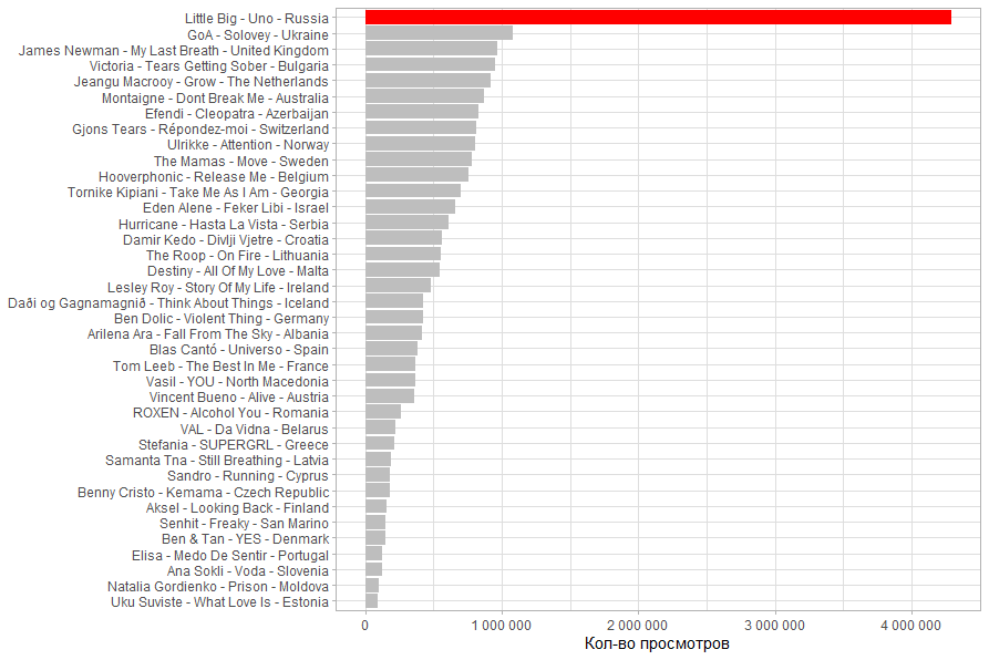
. .
# -
ggplot(df, aes(x = reorder(name_video, viewCount), y = viewCount, fill = color)) +
geom_col() +
coord_flip() +
theme_light() +
labs(x = NULL, y = "- ") +
guides(fill = F) +
scale_fill_manual(values = c('gray', 'red')) +
scale_y_continuous(labels = scales::number_format(big.mark = " "))
#
ggplot(df, aes(x = reorder(name_video, proc_like), y = proc_like, fill = color)) +
geom_col() +
coord_flip() +
theme_light() +
labs(x = NULL, y = " ") +
guides(fill = F) +
scale_fill_manual(values = c('gray', 'red')) +
scale_y_continuous(labels = scales::percent_format(accuracy = 1))
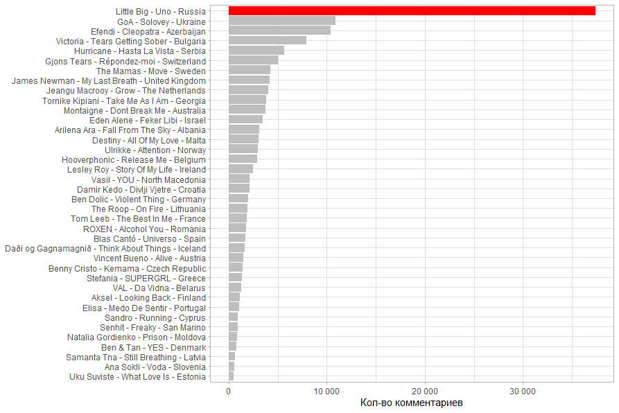
# -
ggplot(df, aes(x = reorder(name_video, commentCount), y = commentCount, fill = color)) +
geom_col() +
coord_flip() +
theme_light() +
labs(x = NULL, y = "- ") +
guides(fill = F) +
scale_fill_manual(values = c('gray', 'red')) +
scale_y_continuous(labels = scales::number_format(big.mark = " "))
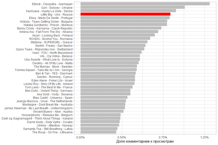
#
ggplot(df, aes(x = reorder(name_video, commentCount/viewCount), y = commentCount/viewCount, fill = color)) +
geom_col() +
coord_flip() +
theme_light() +
labs(x = NULL, y = " ") +
guides(fill = F) +
scale_fill_manual(values = c('gray', 'red')) +
scale_y_continuous(labels = scales::percent_format(accuracy = 0.25))
, Little Big 1 , .
. Little Big , . - .
, . . .

.
( / ). . .
13.03.2020 18:00 , , , .
UPD: 14.03.2020 20:30
. . Little Big , .

, . Little Big ,

.

( / ). 2 , , , . .

14.03.2020 20:30 , , , , . .
:
helg1978 . .
library(rvest)
library(tidyr)

#
hdoc <- read_html('https://en.wikipedia.org/wiki/List_of_countries_and_dependencies_by_population')

tnode <- html_node(hdoc, xpath = '/html/body/div[3]/div[3]/div[4]/div/table')
df_population <- html_table(tnode)

df_population <- df_population %>% filter(`Country (or dependent territory)` != 'World')

df_population$Population <- as.integer(gsub(',','',df_population$Population,fixed = T))

df_population$`Country (or dependent territory)` <- gsub('\\[.*\\]','', df_population$`Country (or dependent territory)`)

df_population <- df_population %>%
  select(
    `Country (or dependent territory)`,
    Population
    ) %>%
  rename(Country = `Country (or dependent territory)`)

#
df2 <- df %>%
  separate(name_video, c('compozitor', 'name_track', 'Country'), ' - ', remove = F) %>%
  mutate(Country = ifelse(Country == 'The Netherlands', 'Netherlands', Country)) %>%
  left_join(df_population, by = 'Country')

#
cor(df2$viewCount,df2$Population)
ggplot(df2, aes(x = Population, y =  viewCount)) +
  geom_point() +
  theme_light() +
  geom_smooth(method = 'lm') +
  labs(x = ", ", y = "- ") +
  scale_y_continuous(labels = scales::number_format(big.mark = " ")) +
  scale_x_continuous(labels = scales::number_format(big.mark = " "))

#     ,
cor(df2[df2$Country != 'Russia',]$viewCount,df2[df2$Country != 'Russia',]$Population)
ggplot(df2 %>% filter(Country != 'Russia') , aes(x = Population, y = viewCount)) +
  geom_point() +
  theme_light() +
  geom_smooth(method = 'lm') +
  labs(x = ", ", y = "- ") +
  scale_y_continuous(labels = scales::number_format(big.mark = " ")) +
  scale_x_continuous(labels = scales::number_format(big.mark = " "))

#     ,
cor(df2$viewCount,df2$Population, method = "spearman")
ggplot(df2 , aes(x = rank(Population), y = rank(viewCount))) +
  geom_point() +
  theme_light() +
  geom_smooth(method = 'lm') +
  labs(x = ",  (  1  40)", y = "-  (  1  40)") +
  guides(fill = F)

#
ggplot(df2, aes(x = reorder(name_video, viewCount/Population), y = viewCount/Population, fill = color)) +
  geom_col() +
  coord_flip() +
  theme_light() +
  labs(x = NULL, y = "    ") +
  guides(fill = F) +
  scale_fill_manual(values = c('gray', 'red')) +
  scale_y_continuous(labels = scales::percent_format(accuracy = 0.25))
, , 50 . 71%.

. 71% 15%. .

( ), , (. . 40%).

And for reference I calculated the share of views from the country's population. For especially small countries, it turns out that they were watched more from other countries. In particular, it is Malta, San Marino and Iceland.

Full github code