🥨 🖌️ 🎪 5 little-known secrets of Pandas 🚲 👩🏽‍💻 📓

Pandas needs no introduction: today it is the main tool for analyzing data in Python. I work as a data analysis specialist, and despite the fact that I use pandas every day, I never cease to be surprised at the variety of functionality of this library. In this article I want to talk about five little-known pandas functions that I recently learned and now use productively.

For beginners: Pandas is a high-performance toolkit for data analysis in Python with simple and convenient data structures. The name comes from the concept of “panel data”, an econometric term that refers to data on observations of the same subjects over different periods of time.

Here you can download the Jupyter Notebook with examples from the article.

1. Date Ranges [Date Ranges]

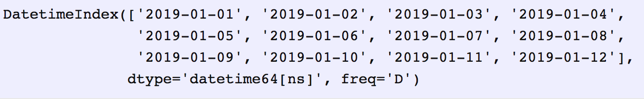
Often you need to specify date ranges when requesting data from an external API or database. Pandas won't leave us in trouble. Just for these cases, there is the data_range function , which returns an array of dates increased by days, months, years, etc.

Say we need a date range by day:

date_from = "2019-01-01"
date_to = "2019-01-12"
date_range = pd.date_range(date_from, date_to, freq="D")
date_range

We will transform the generated from date_rangeinto pairs of dates “from” and “to”, which can be transferred to the corresponding function.

for i, (date_from, date_to) in enumerate(zip(date_range[:-1], date_range[1:]), 1):
   date_from = date_from.date().isoformat()
   date_to = date_to.date().isoformat()
   print("%d. date_from: %s, date_to: %s" % (i, date_from, date_to))

1. date_from: 2019-01-01, date_to: 2019-01-02
2. date_from: 2019-01-02, date_to: 2019-01-03
3. date_from: 2019-01-03, date_to: 2019-01-04
4. date_from: 2019-01-04, date_to: 2019-01-05
5. date_from: 2019-01-05, date_to: 2019-01-06
6. date_from: 2019-01-06, date_to: 2019-01-07
7. date_from: 2019-01-07, date_to: 2019-01-08
8. date_from: 2019-01-08, date_to: 2019-01-09
9. date_from: 2019-01-09, date_to: 2019-01-10
10. date_from: 2019-01-10, date_to: 2019-01-11
11. date_from: 2019-01-11, date_to: 2019-01-12

2. Merge with the source indicator [Merge with indicator]

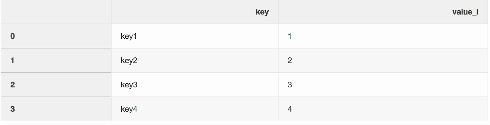
Merging two datasets is, oddly enough, the process of combining two datasets into one whose rows are mapped based on common columns or properties.

One of the two arguments to the merge function, which I somehow missed, is indicator. The “Indicator” adds a column _mergeto the DataFrame that shows where the row came from, from left, right, or both DataFrames. A column _mergecan be very useful when working with large data sets to verify the merge is correct.

left = pd.DataFrame({"key": ["key1", "key2", "key3", "key4"], "value_l": [1, 2, 3, 4]})

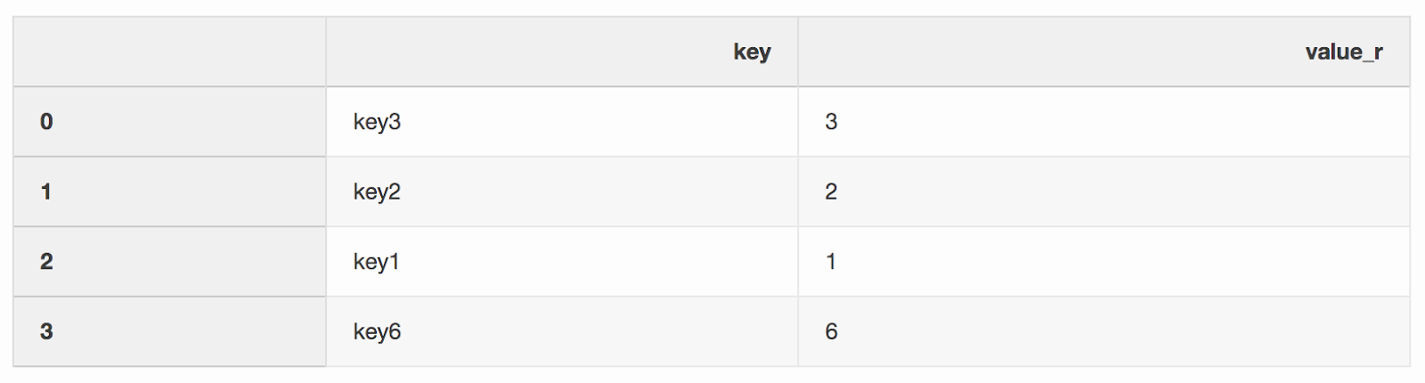
right = pd.DataFrame({"key": ["key3", "key2", "key1", "key6"], "value_r": [3, 2, 1, 6]})

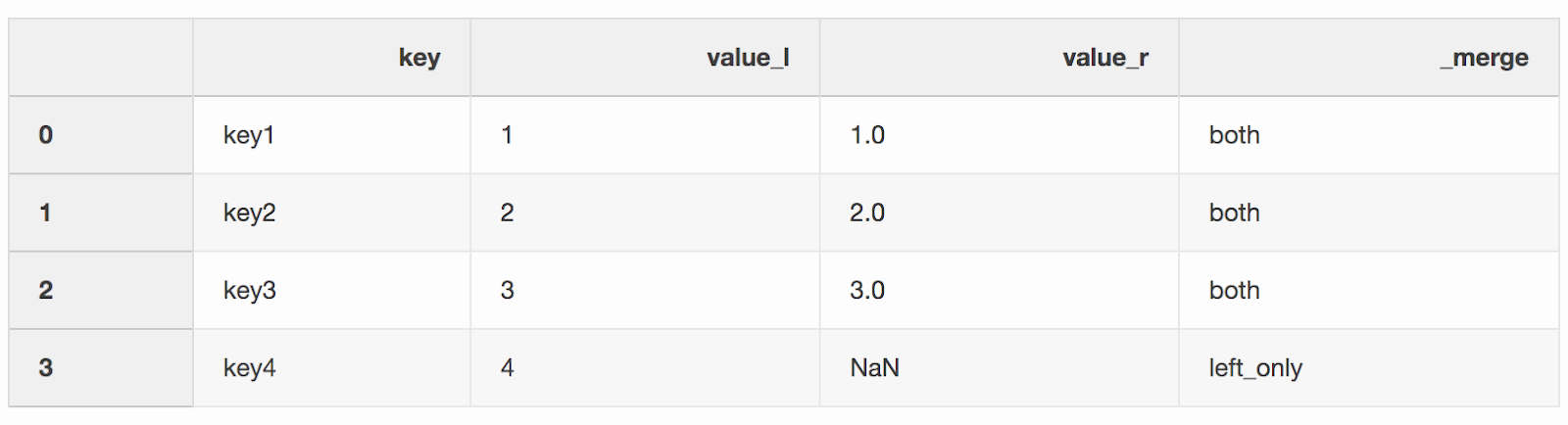
df_merge = left.merge(right, on='key', how='left', indicator=True)

The column _mergecan be used to check if the correct number of rows with data was taken from both DataFrames.

df_merge._merge.value_counts()

both          3
left_only     1
right_only    0
Name: _merge, dtype: int64

3. Merge by the closest value [Nearest merge]

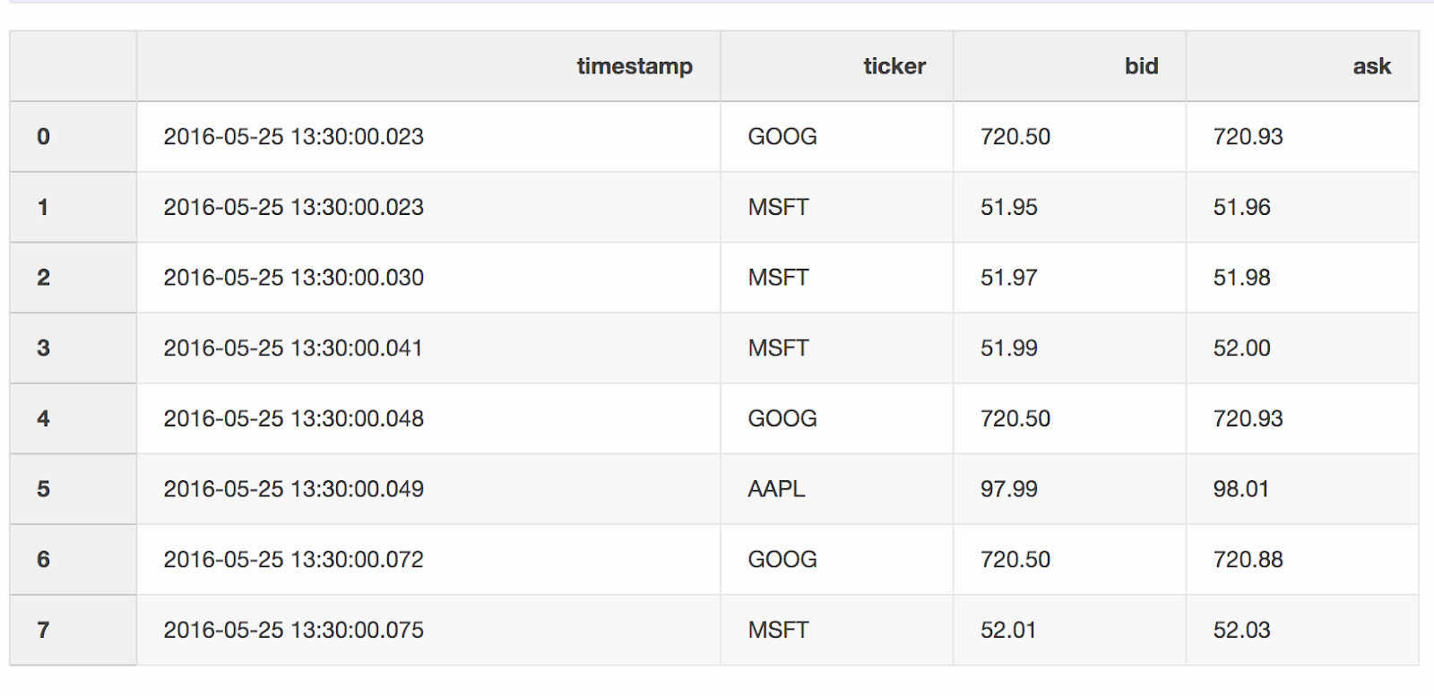
When working with financial data, such as cryptocurrencies and securities, it may be necessary to compare quotes (price changes) with transactions. Let's say we want to combine every trade with a quote that was updated a few milliseconds before the trade. Pandas has a function merge_asofdue to which it is possible to combine DataFrames by the closest key value ( timestampin our case). Data sets with quotes and deals are taken from pandas example .

DataFrame quotes(“quotes”) contains price changes for different stocks. As a rule, there are much more quotes than deals.

quotes = pd.DataFrame(
   [
       ["2016-05-25 13:30:00.023", "GOOG", 720.50, 720.93],
       ["2016-05-25 13:30:00.023", "MSFT", 51.95, 51.96],
       ["2016-05-25 13:30:00.030", "MSFT", 51.97, 51.98],
       ["2016-05-25 13:30:00.041", "MSFT", 51.99, 52.00],
       ["2016-05-25 13:30:00.048", "GOOG", 720.50, 720.93],
       ["2016-05-25 13:30:00.049", "AAPL", 97.99, 98.01],
       ["2016-05-25 13:30:00.072", "GOOG", 720.50, 720.88],
       ["2016-05-25 13:30:00.075", "MSFT", 52.01, 52.03],
   ],
   columns=["timestamp", "ticker", "bid", "ask"],
)
quotes['timestamp'] = pd.to_datetime(quotes['timestamp'])

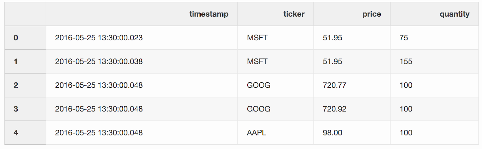
DataFrame tradescontains deals for different stocks.

trades = pd.DataFrame(
   [
       ["2016-05-25 13:30:00.023", "MSFT", 51.95, 75],
       ["2016-05-25 13:30:00.038", "MSFT", 51.95, 155],
       ["2016-05-25 13:30:00.048", "GOOG", 720.77, 100],
       ["2016-05-25 13:30:00.048", "GOOG", 720.92, 100],
       ["2016-05-25 13:30:00.048", "AAPL", 98.00, 100],
   ],
   columns=["timestamp", "ticker", "price", "quantity"],
)
trades['timestamp'] = pd.to_datetime(trades['timestamp'])

We merge transactions and quotes by tickers (a quoted instrument, such as stocks), provided that the timestamplast quote may be 10 ms less than the transaction. If the quote appeared before the transaction for more than 10 ms, the bid (the price that the buyer is ready to pay) and ask (the price at which the seller is ready to sell) for this quote will be null(AAPL ticker in this example).

pd.merge_asof(trades, quotes, on="timestamp", by='ticker', tolerance=pd.Timedelta('10ms'), direction='backward')

4. Creating an Excel report

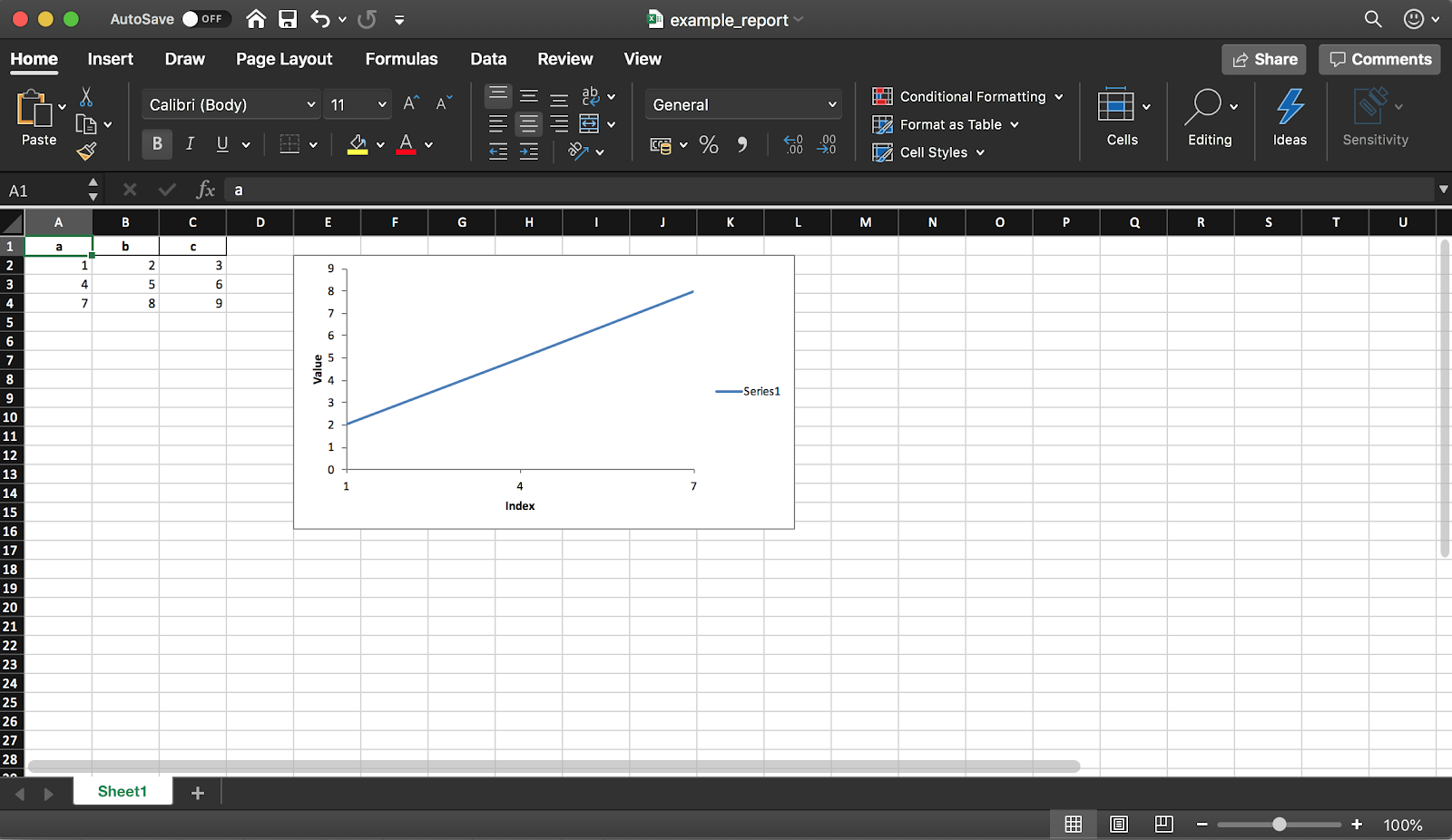Pandas (with the XlsxWriter library) allows you to create an Excel report from a DataFrame. This saves you a ton of time - no more exporting a DataFrame to CSV and manual formatting to Excel. All kinds of diagrams , etc. are also available .

df = pd.DataFrame(pd.np.array([[1, 2, 3], [4, 5, 6], [7, 8, 9]]), columns=["a", "b", "c"])

The code snippet below creates a table in Excel format. Uncomment the line to save it to a file writer.save().

report_name = 'example_report.xlsx'
sheet_name = 'Sheet1'
writer = pd.ExcelWriter(report_name, engine='xlsxwriter')
df.to_excel(writer, sheet_name=sheet_name, index=False)
# writer.save()

As mentioned earlier, using the library you can also add charts to the report. You need to specify the type of chart (linear in our example) and the data range for it (the data range should be in the Excel table).

#   (workbook)
workbook = writer.book
worksheet = writer.sheets[sheet_name]
#   
chart = workbook.add_chart({'type': 'line'})
#       ,
#      /:
#     [sheetname, first_row, first_col, last_row, last_col]
chart.add_series({
   'categories': [sheet_name, 1, 0, 3, 0],
   'values':     [sheet_name, 1, 1, 3, 1],
})
#   
chart.set_x_axis({'name': 'Index', 'position_axis': 'on_tick'})
chart.set_y_axis({'name': 'Value', 'major_gridlines': {'visible': False}})
#    
worksheet.insert_chart('E2', chart)
#  
writer.save()

5. Save disk space

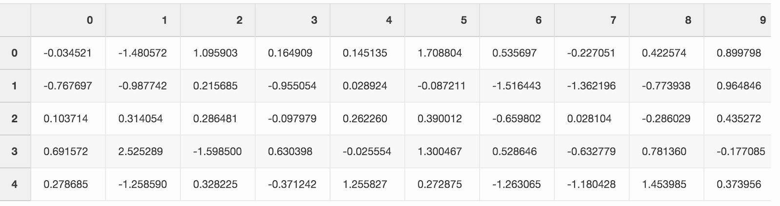
Work on a large number of data analysis projects usually leaves a mark in the form of a large amount of processed data from various experiments. The SSD on the laptop fills up pretty quickly. Pandas allows you to compress data while saving data to disk and then read it again from a compressed format.

Create a large DataFrame with random numbers.

df = pd.DataFrame(pd.np.random.randn(50000,300))

If you save it as a CSV, the file will take up almost 300 MB on your hard drive.

df.to_csv('random_data.csv', index=False)

One argument compression='gzip'reduces the file size to 136 MB.

df.to_csv('random_data.gz', compression='gzip', index=False)

A compressed file is read in the same way as a regular file, so we do not lose any functionality.

df = pd.read_csv('random_data.gz')

Conclusion

These little tricks have increased the productivity of my daily work with pandas. I hope you learned from this article about some useful feature that will help you become more productive as well.

What is your favorite trick with pandas?