When studying Data Science, I decided to compile for myself a summary of the basic techniques used in data analysis. It reflects the names of the methods, briefly describes the essence and provides Python code for quick application. I was preparing a compendium for myself, but I thought that it might also be useful to someone, for example, before an interview, in a competition, or when starting a new project. Designed for an audience that is generally familiar with all these methods, but has the need to refresh them in memory. Article under the cut.- Naive Bayes classifier . The formula for calculating the probability of classifying an observation as one or another class:
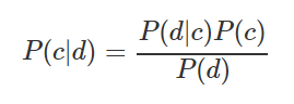
For example, you need to calculate the probability that a sports match will take place provided that the weather is sunny. The source data and calculations are shown in the table below: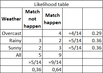
You can calculate by the formula (3/9) * (9/14) / (5/14) = 60%, or just from common sense 3 / (2 + 3) = 60%. Strengths - easy to interpret the result, suitable for large samples and multi-class classification. Weaknesses - the assumption that the characteristics are independent is not always fulfilled; characteristics should make up a complete group of events.
from sklearn.datasets import load_iris
from sklearn.model_selection import train_test_split
from sklearn.naive_bayes import GaussianNB
X, y = load_iris(return_X_y=True)
X_train, X_test, y_train, y_test = train_test_split(X, y, test_size=0.5, random_state=0)
gnb = GaussianNB()
y_pred = gnb.fit(X_train, y_train).predict(X_test)
print("Number of mislabeled points out of a total %d points : %d"
% (X_test.shape[0], (y_test != y_pred).sum()))
- Method of nearest neighbors . Classifies each observation according to the degree of similarity to other observations. The algorithm is nonparametric (there are no restrictions on the data, for example, the distribution function) and uses lazy training (pre-trained models are not used, all available data are used during classification).
Strengths - easy to interpret the result, well suited for tasks with a small number of explanatory variables. Weaknesses - low accuracy compared to other methods. It requires significant computing power with a large number of explanatory variables and large samples.
from sklearn.neighbors import KNeighborsClassifier
X = [[0], [1], [2], [3]]
y = [0, 0, 1, 1]
neigh = KNeighborsClassifier(n_neighbors=3)
neigh.fit(X, y)
print(neigh.predict([[1.1]]))
print(neigh.predict_proba([[0.9]]))
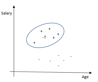
- Support Vector Method (SVM) . Each data object is represented as a vector (point) in p-dimensional space. The task is to separate the points with a hyperplane. That is, is it possible to find such a hyperplane so that the distance from it to the nearest point is maximum. There can be many sought-after hyperplanes; therefore, it is believed that maximizing the gap between classes contributes to a more confident classification.
— . , , . . — , , , , . .
from sklearn import svm
X = [[0, 0], [1, 1]]
y = [0, 1]
clf = svm.SVC()
clf.fit(X, y)
clf.predict([[2., 2.]])
- Decision trees . Dividing data into subsamples according to a certain condition in the form of a tree structure. Mathematically, the division into classes occurs until all the conditions that determine the class as precisely as possible are found, i.e., when there are no representatives of another class in each class. In practice, a limited number of characteristics and layers are used, and there are always two branches.

Strengths - it is possible to simulate complex processes and easily interpret them. Multiclass classification is possible. Weaknesses - it is easy to retrain the model if you make many layers. Emissions can affect accuracy; the solution to these problems is to trim the lower levels.
from sklearn.datasets import load_iris
from sklearn import tree
X, y = load_iris(return_X_y=True)
clf = tree.DecisionTreeClassifier()
clf = clf.fit(X, y)
tree.plot_tree(clf.fit(iris.data, iris.target))
- / . . — . (random patching) . oob-.
: , , , , , . , . — , . , ( 100 000), — .
from sklearn.ensemble import RandomForestClassifier
from sklearn.datasets import make_classification
X, y = make_classification(n_samples=1000, n_features=4,
n_informative=2, n_redundant=0,
random_state=0, shuffle=False)
clf = RandomForestClassifier(max_depth=2, random_state=0)
clf.fit(X, y)
print(clf.feature_importances_)
print(clf.predict([[0, 0, 0, 0]]))
- . ( hinge loss function). .
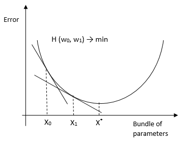
There is also a version of stochastic gradient descent, which is used for large samples. Its essence is that it considers the derivative not for the entire sample, but for each observation (online learning) (or for the mini-batch observation group) and changes weights. As a result, he comes to the same optimum as with a conventional HS. There are methods of using HS for OLS, logit, tobit and other methods ( evidence ).Strengths : high accuracy of classification and forecasting, suitable for multi-class classification. Weaknesses - sensitivity to model parameters.
from sklearn.linear_model import SGDClassifier
X = [[0., 0.], [1., 1.]]
y = [0, 1]
clf = SGDClassifier(loss="hinge", penalty="l2", max_iter=5)
clf.fit(X, y)
clf.predict([[2., 2.]])
clf.coef_
clf.intercept_
- . . , . , , .
: , , , . — .
import numpy as np
import matplotlib.pyplot as plt
from sklearn import ensemble
from sklearn import datasets
from sklearn.utils import shuffle
from sklearn.metrics import mean_squared_error
boston = datasets.load_boston()
X, y = shuffle(boston.data, boston.target, random_state=13)
X = X.astype(np.float32)
offset = int(X.shape[0] * 0.9)
X_train, y_train = X[:offset], y[:offset]
X_test, y_test = X[offset:], y[offset:]
params = {'n_estimators': 500, 'max_depth': 4, 'min_samples_split': 2,
'learning_rate': 0.01, 'loss': 'ls'}
clf = ensemble.GradientBoostingRegressor(**params)
clf.fit(X_train, y_train)
mse = mean_squared_error(y_test, clf.predict(X_test))
print("MSE: %.4f" % mse)
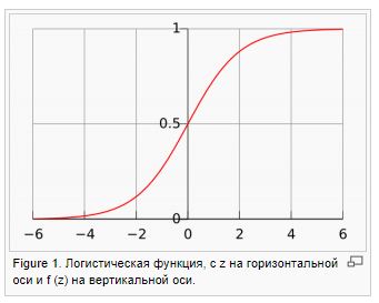
- /logit. 0 1, (log likelihood). — Y w.

: , . — , .
from sklearn.datasets import load_iris
from sklearn.linear_model import LogisticRegression
X, y = load_iris(return_X_y=True)
clf = LogisticRegression(random_state=0).fit(X, y)
clf.predict(X[:2, :])
clf.predict_proba(X[:2, :])
clf.score(X, y)
-Probit. , , , .
import statsmodels
result_3 = statsmodels.discrete.
discrete_model.Probit(labf_part, ind_var_probit )
print(result_3.summary())
-Tobit. , .
from sklearn.datasets import make_regression
import matplotlib.pyplot as plt
import pandas as pd
from tobit import *
tr = TobitModel()
tr = tr.fit(x, y, cens, verbose=False)
tr.coef_
- , , . , , , . .