Hello, Habr!We remind you that earlier we announced the book " Machine Learning Without Extra Words " - and now it is already on sale . Despite the fact that for beginners in MO, the book can indeed become a desktop , some topics in it still were not touched. Therefore, we are offering everyone interested a translation of an article by Simon Kerstens on the essence of MCMC algorithms with the implementation of such an algorithm in Python.Monte Carlo methods for Markov chains (MCMC) are a powerful class of methods for sampling from probability distributions that are known only up to a certain (unknown) normalization constant.However, before delving into the MCMC, let's discuss why you might even need to make such a selection. The answer is: you may be interested in either the samples themselves from the sample (for example, to determine unknown parameters using the Bayesian derivation method), or to approximate the expected values of the functions relative to the probability distribution (for example, to calculate thermodynamic quantities from the distribution of states in statistical physics). Sometimes we are only interested in the probability distribution mode. In this case, we obtain it by the method of numerical optimization, so it is not necessary to make a complete selection.It turns out that sampling from any probability distributions except the most primitive ones is a difficult task. The inverse transformation method is an elementary technique for sampling from probability distributions, which, however, requires the use of a cumulative distribution function, and to use it, in turn, you need to know the normalization constant, which is usually unknown. In principle, a normalization constant can be obtained by numerical integration, but this method quickly becomes impracticable with an increase in the number of dimensions. Deviation SamplingIt does not require a normalized distribution, but in order to effectively implement it, it takes a lot to know about the distribution of interest to us. In addition, this method suffers severely from the curse of dimensions - this means that its effectiveness rapidly decreases with an increase in the number of variables. That is why you need to intelligently organize the receipt of representative samples from your distribution - not requiring to know the normalization constant.MCMC algorithms are a class of methods designed specifically for this. They go back to the landmark article of Metropolis and others ; Metropolis developed the first MCMC algorithm named after himand designed to calculate the equilibrium state of a two-dimensional system of hard spheres. In fact, the researchers were looking for a universal method that would allow us to calculate the expected values found in statistical physics.This article will cover the basics of MCMC sampling.MARKOV CHAINSNow that we understand why we need to sample, let's move on to the heart of MCMC: Markov chains. What is a Markov chain? Without going into technical details, we can say that a Markov chain is a random sequence of states in a certain state space, where the probability of choosing a certain state depends only on the current state of the chain, but not on its past history: this chain is devoid of memory. Under certain conditions, a Markov chain has a unique stationary distribution of states, to which it converges, overcoming a certain number of states. After such a number of state states in a Markov chain, an invariant distribution is obtained.To sample from a distribution,  the MCMC algorithm creates and simulates a Markov chain whose stationary distribution is; this means that after the initial “seed” period, the states of such a Markov chain are distributed according to the principle . Therefore, we will only have to save the state in order to get samples from .For educational purposes, let us consider both a discrete state space and a discrete “time”. The key quantity characterizing a Markov chain is a transition operator
  indicating the probability of being in a state
  at a time
  , provided that the chain is in a state at time
 i.Now just for fun (and as a demonstration) let's quickly weave a Markov chain with a unique stationary distribution. Let's start with some imports and settings for charts:%matplotlib notebook
%matplotlib inline
import numpy as np
import matplotlib.pyplot as plt
plt.rcParams['figure.figsize'] = [10, 6]
np.random.seed(42)
The Markov chain will go around the discrete state space formed by three weather conditions:state_space = ("sunny", "cloudy", "rainy")
In a discrete state space, the transition operator is just a matrix. In our case, the columns and rows correspond to sunny, cloudy and rainy weather. Let us choose relatively reasonable values for the probabilities of all transitions:transition_matrix = np.array(((0.6, 0.3, 0.1),
(0.3, 0.4, 0.3),
(0.2, 0.3, 0.5)))
The rows indicate the states in which the circuit may currently be located, and the columns indicate the states into which the circuit can go. If we take the “time” step of the Markov chain in one hour, then, provided that it is sunny now, there is a 60% chance that the sunny weather will continue for the next hour. There is also a 30% chance that there will be cloudy weather in the next hour, and a 10% chance that it will rain immediately after sunny weather. It also means that the values in each row add up to one.Let's drive our Markov chain a little:n_steps = 20000
states = [0]
for i in range(n_steps):
states.append(np.random.choice((0, 1, 2), p=transition_matrix[states[-1]]))
states = np.array(states)
We can observe how the Markov chain converges to a stationary distribution, calculating the empirical probability of each of the states as a function of chain length:def despine(ax, spines=('top', 'left', 'right')):
for spine in spines:
ax.spines[spine].set_visible(False)
fig, ax = plt.subplots()
width = 1000
offsets = range(1, n_steps, 5)
for i, label in enumerate(state_space):
ax.plot(offsets, [np.sum(states[:offset] == i) / offset
for offset in offsets], label=label)
ax.set_xlabel("number of steps")
ax.set_ylabel("likelihood")
ax.legend(frameon=False)
despine(ax, ('top', 'right'))
plt.show()
 HONOR OF ALL MCMC: METROPOLIS-HASTINGS ALGORITHMOf course, all this is very interesting, but back to the sampling process of an arbitrary probability distribution
  . It can be either discrete, in which case we will continue to talk about the transition matrix
  , or continuous, in which case it will be a transition core. Hereinafter, we will talk about continuous distributions, but all the concepts that we consider here are also applicable to discrete cases.If we could design the transition core in such a way that the next state was already deduced from , then this could be limited, since our Markov chain ... would directly sample from . Unfortunately, to achieve this, we need the ability to sample fromwhat we cannot do - otherwise you would not read that, right?The workaround is to break the transition core
  into two parts: the proposal step and the acceptance / rejection step. An auxiliary distribution appears at the sample step
 from which the possible next states of the chain are selected. Not only can we make a selection from this distribution, but we can arbitrarily choose the distribution itself. However, when designing, one should strive to come to such a configuration in which samples taken from this distribution would be minimally correlated with the current state and at the same time have good chances to go through the receiving phase. The above receiving / discarding step is the second part of the transition core; at this stage, errors contained in the trial states selected from are corrected
  . Here, the probability of successful reception is calculated
  and a sample is taken with such probability as the next state in the chain. Getting the next state fromthen performed as follows: first, the trial state is taken from . Then it is taken as the next state with probability or discarded with probability
  , and in the latter case, the current state is copied and used as the next.Consequently, we have
 sufficient condition for the Markov chain had as a stationary distribution is the following: The transitional core must submit detailed equilibrium or as write in the physical literature, microscopic reversibility :
 .This means that the probability of being in a state
  and moving from there to
 must be equal to the probability of the reverse process, that is, be able to and go into a state . The transition kernels of most MCMC algorithms satisfy this condition.In order for the two-part transition core to obey detailed equilibrium, it is necessary to choose correctly
  , that is, to ensure that it allows you to correct any asymmetries in the probability stream from / to or . Metropolis-Hastings algorithm uses admissibility criterion Metropolis:
 .And here the magic begins: we know only to a constant, but it does not matter, since this unknown constant nullifies the expression for! It is this paccpacc property that ensures the operation of algorithms based on the Metropolis-Hastings algorithm on unnormalized distributions. Symmetric auxiliary distributions c are often used
  , in which case the Metropolis-Hastings algorithm is reduced to the original (less general) Metropolis algorithm developed in 1953. In the original algorithm
 .In this case, the complete transitional core of the Metropolis-Hastings can be written as
 .WE IMPLEMENT THE METROPOLIS-HASTINGS ALGORITHM AT PYTHONGreat, now that we’ve figured out how the Metropolis-Hastings algorithm works, let's move on to its implementation. First, we establish the logarithmic probability of the distribution from which we are going to make a selection - without normalization constants; it is assumed that we do not know them. Next, we work with the standard normal distribution:
def log_prob(x):
     return -0.5 * np.sum(x ** 2)
Next, we choose a symmetric auxiliary distribution. In general, the performance of the Metropolis-Hastings algorithm can be improved if you include information already known to you about the distribution from which you want to make a selection in the auxiliary distribution. A simplified approach looks like this: we take the current state xand select a sample from , that is, set a certain step size Δand go left or right from our current state by no more than  :
:def proposal(x, stepsize):
return np.random.uniform(low=x - 0.5 * stepsize,
high=x + 0.5 * stepsize,
size=x.shape)
Finally, we calculate the probability that the proposal will be accepted:def p_acc_MH(x_new, x_old, log_prob):
return min(1, np.exp(log_prob(x_new) - log_prob(x_old)))
Now we put all this together into a truly brief implementation of the sampling stage for the Metropolis-Hastings algorithm:def sample_MH(x_old, log_prob, stepsize):
x_new = proposal(x_old, stepsize)
accept = np.random.random() < p_acc(x_new, x_old, log_prob)
if accept:
return accept, x_new
else:
return accept, x_old
In addition to the next state in the Markov chain, x_newor x_old, we also return information about whether the MCMC step was adopted. This will allow us to track the dynamics of sample collection. In conclusion of this implementation, we write a function that will iteratively call sample_MHand thus build a Markov chain:def build_MH_chain(init, stepsize, n_total, log_prob):
n_accepted = 0
chain = [init]
for _ in range(n_total):
accept, state = sample_MH(chain[-1], log_prob, stepsize)
chain.append(state)
n_accepted += accept
acceptance_rate = n_accepted / float(n_total)
return chain, acceptance_rate
TESTING OUR METROPOLIS-HASTINGS ALGORITHM AND RESEARCHING ITS BEHAVIORProbably, now you can not wait to see all this in action. We will do this, we will make some informed decisions about the arguments stepsizeand n_total:chain, acceptance_rate = build_MH_chain(np.array([2.0]), 3.0, 10000, log_prob)
chain = [state for state, in chain]
print("Acceptance rate: {:.3f}".format(acceptance_rate))
last_states = ", ".join("{:.5f}".format(state)
for state in chain[-10:])
print("Last ten states of chain: " + last_states)
Acceptance rate: 0.722
Last ten states of chain: -0.84962, -0.84962, -0.84962, -0.08692, 0.92728, -0.46215, 0.08655, -0.33841, -0.33841, -0.33841
Things are good. So, did it work? We succeeded in taking samples in about 71% of cases, and we have a chain of states. The first few states in which the chain has not yet converged to its stationary distribution should be discarded. Let's check if the conditions we have chosen actually have a normal distribution:def plot_samples(chain, log_prob, ax, orientation='vertical', normalize=True,
xlims=(-5, 5), legend=True):
from scipy.integrate import quad
ax.hist(chain, bins=50, density=True, label="MCMC samples",
orientation=orientation)
if normalize:
Z, _ = quad(lambda x: np.exp(log_prob(x)), -np.inf, np.inf)
else:
Z = 1.0
xses = np.linspace(xlims[0], xlims[1], 1000)
yses = [np.exp(log_prob(x)) / Z for x in xses]
if orientation == 'horizontal':
(yses, xses) = (xses, yses)
ax.plot(xses, yses, label="true distribution")
if legend:
ax.legend(frameon=False)
fig, ax = plt.subplots()
plot_samples(chain[500:], log_prob, ax)
despine(ax)
ax.set_yticks(())
plt.show()
 It looks great!What about the parameters
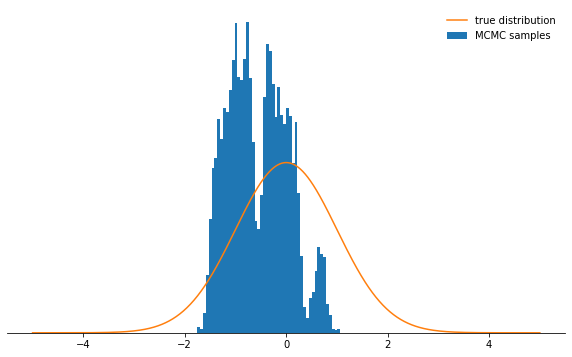
 stepsizeand n_total? We first discuss the step size: it determines how far the trial state can be removed from the current state of the circuit. Therefore, this is an auxiliary distribution parameter qthat controls how large the random steps taken by the Markov chain will be. If the step size is too large, the trial states often end up in the tail of the distribution, where the probability values are low. The Metropolis-Hastings sampling mechanism discards most of these steps, as a result of which reception rates are reduced and convergence slows significantly. See for yourself:def sample_and_display(init_state, stepsize, n_total, n_burnin, log_prob):
chain, acceptance_rate = build_MH_chain(init_state, stepsize, n_total, log_prob)
print("Acceptance rate: {:.3f}".format(acceptance_rate))
fig, ax = plt.subplots()
plot_samples([state for state, in chain[n_burnin:]], log_prob, ax)
despine(ax)
ax.set_yticks(())
plt.show()
sample_and_display(np.array([2.0]), 30, 10000, 500, log_prob)
Acceptance rate: 0.116
 Not very cool, right? Now it seems that it's best to set a tiny step size. It turns out that this is not a smart decision either, since the Markov chain will investigate the probability distribution very slowly, and therefore also will not converge as quickly as with a well-chosen step size:
sample_and_display(np.array([2.0]), 0.1, 10000, 500, log_prob)
Acceptance rate: 0.992
 Regardless of how you choose the step size parameter, the Markov chain eventually converges to a stationary distribution. But this may take a lot of time. The time during which we will simulate the Markov chain is
 n_totaldetermined by the parameter - it simply determines how many states of the Markov chain (and, therefore, the selected samples) we will eventually have. If the chain converges slowly, then it needs to be increased n_totalso that the Markov chain has time to “forget” the initial state. Therefore, we will leave the step size tiny and increase the number of samples by increasing the parameter n_total:sample_and_display(np.array([2.0]), 0.1, 500000, 25000, log_prob)
Acceptance rate: 0.990
 Meeeedenly we are moving towards the goal ...CONCLUSIONSConsidering all the above, I hope that now you have intuitively grasped the essence of the Metropolis-Hastings algorithm, its parameters, and understand why this is an extremely useful tool for selecting from non-standard probability distributions that you may encounter in practice.I strongly recommend that you experiment with the code given here.- so you get used to the behavior of the algorithm in various circumstances and understand it more deeply. Try asymmetric auxiliary distribution! What will happen if you do not configure the acceptance criterion properly? What happens if you try to sample from a bimodal distribution? Can you come up with a way to automatically adjust the step size? What are the pitfalls here? Answer these questions yourself!