 Hello everyone!Engaged in performance testing. And I really like to set up monitoring and enjoy the metrics in Grafana . And the standard for storing metrics in load tools is InfluxDB . In InfluxDB, you can save metrics from such popular tools as:Working with performance testing tools and their metrics, I have accumulated a selection of programming recipes for the bundle of Grafana and InfluxDB . I propose to consider an interesting problem that arises where there is a metric with two or more tags. I think this is not uncommon. And in the general case, the task sounds like this: calculating the total metric for a group, which is divided into subgroups .
There are three options:
- Just the amount grouped by Type tag
- Grafana-way. We use a stack of values
- Sum of highs with subquery
How it all began
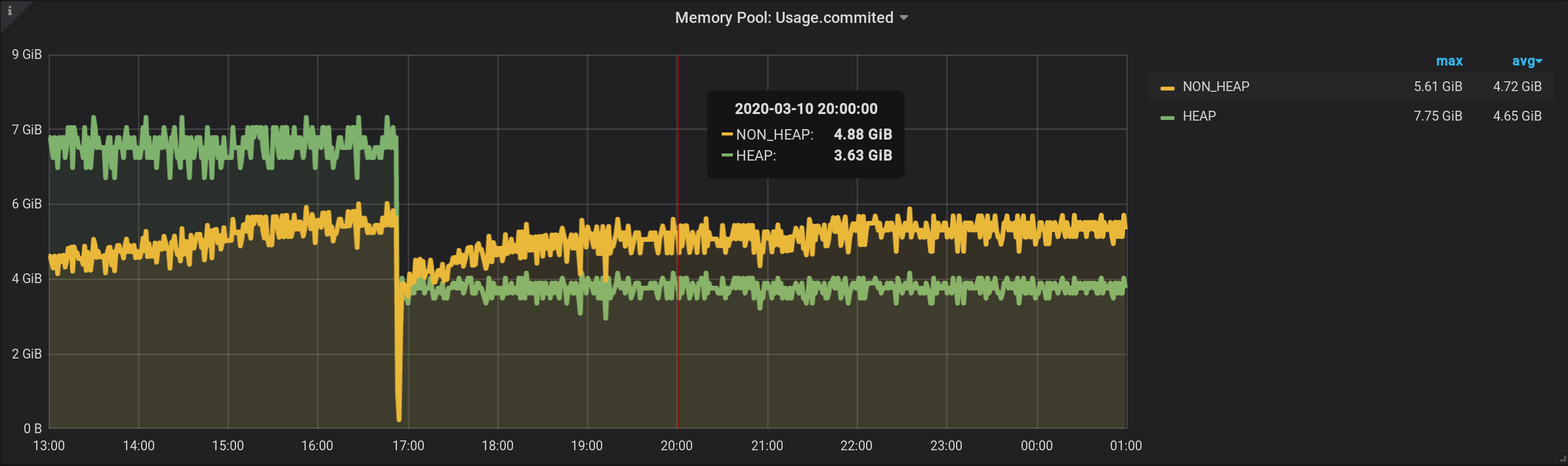
Configured JVM MBean monitoring using Jolokia , Telegraf , InfluxDB and Grafana . And he visualized metrics on memory pools - how much memory is allocated by each memory pool in HEAP and beyond.Charts on JVM memory pools and garbage collector activity from 13:00 of the previous day to 01:00 of the night of the current day (period of 12 hours). Here you can see that the memory pools are divided into two groups: HEAP and NON_HEAP . And that around 17:00 there was garbage collection, after which the size of the memory pools decreased: To collect metrics on memory pools, I specified the following settings in the telegraf configuration file : telegraf.conf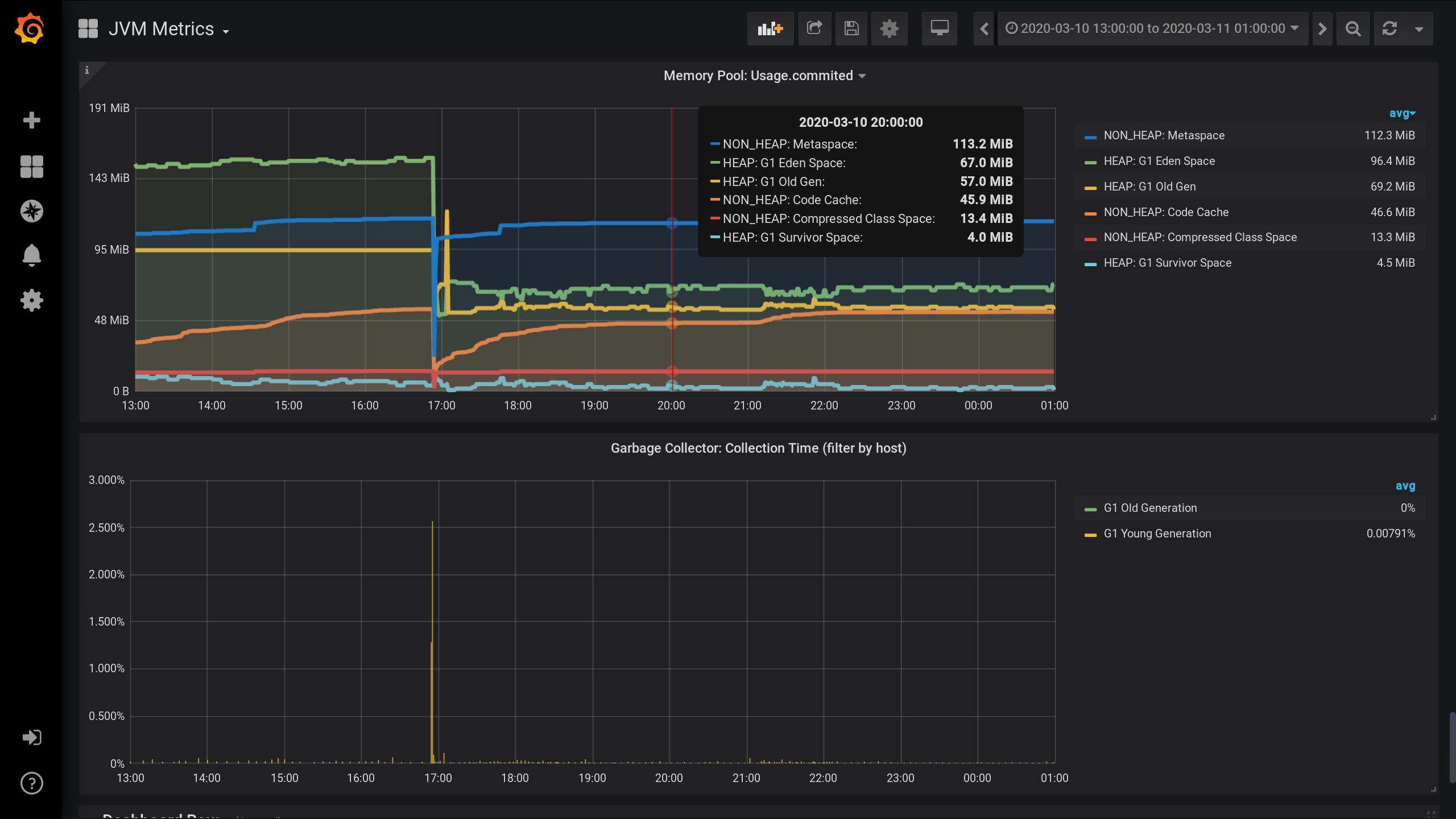
[outputs.influxdb]
  urls = ["http://influxdb_server:8086"]
  database = "telegraf"
  username = "login-InfluxDb"
  password = "*****"
  retention_policy = "month"
  influx_uint_support = false

[agent]
  collection_jitter = "2s"
  interval = "2s"
  precision = "s"

[[inputs.jolokia2_agent]]
  username = "login-Jolokia"
  password = "*****"
  urls = ["http://127.0.0.1:7777/jvm-service"]

[[inputs.jolokia2_agent.metric]]
  paths = ["Usage","PeakUsage","CollectionUsage","Type"]
  name = "java_memory_pool"
  mbean = "java.lang:name=*,type=MemoryPool"
  tag_keys = ["name"]

[[processors.converter]]
  [processors.converter.fields]
    integer = ["CollectionUsage.*", "PeakUsage.*", "Usage.*"]
    tag = ["Type"]
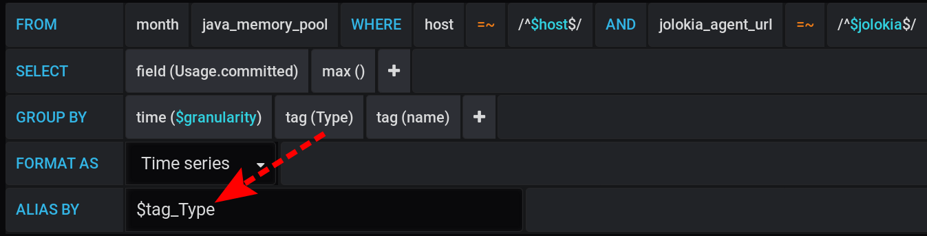
And in Grafana, I constructed a query to InfluxDB to display in graphs the maximum metric value Usage.Committedfor a period of time with a step $granularity(1m) and grouped by two tags Type(HEAP or NON_HEAP) and name(Metaspace, G1 Old Gen, ...): The same query in text form, taking into account all Grafana variables (pay attention to escaping variable values with - this is important for the query to work correctly):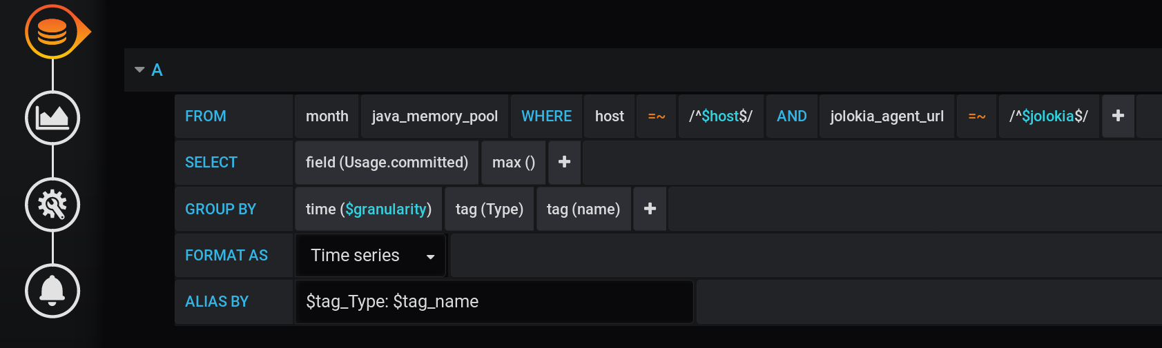
:regexSELECT max("Usage.committed")
FROM "telegraf"."month"."java_memory_pool"
WHERE
host =~ /^${host:regex}$/ AND
jolokia_agent_url =~ /^${jolokia:regex}$/ AND
$timeFilter
GROUP BY
"Type", "name", time($granularity)
The same query in text form, taking into account the specific values of Grafana variables :SELECT max("Usage.committed")
FROM "telegraf"."month"."java_memory_pool"
WHERE
host =~ /^serverName$/ AND
jolokia_agent_url =~ /^http:\/\/127\.0\.0\.1:7777\/jvm-service$/ AND
time >= 1583834400000ms and time <= 1583877600000ms
GROUP BY
"Type", "name", time(1m)
Grouping by time GROUP BY time($granularity)or is GROUP BY time(1m)used to reduce the number of points on the chart. For a time period of 12 hours and a grouping step of 1 minute, we get: 12 x 60 = 720 times or 721 points (the last point with a value of null).Remember that 721 is the expected number of points in response to requests to InfluxDB with the current settings for the time interval (12 hours) and grouping step (1 minute).
NON_HEAP
memory pool: Metaspace (blue) is in the lead in memory consumption at 20:00. And according to HEAP: G1 Old Gen (yellow) there was a small local surge at 17:03. And at the time of 20:00, in total, all NON_HEAP pools left 172.5 MiB (113.2 + 45.9 + 13.4), and HEAP pools 128 MiB (67 + 57 + 4).
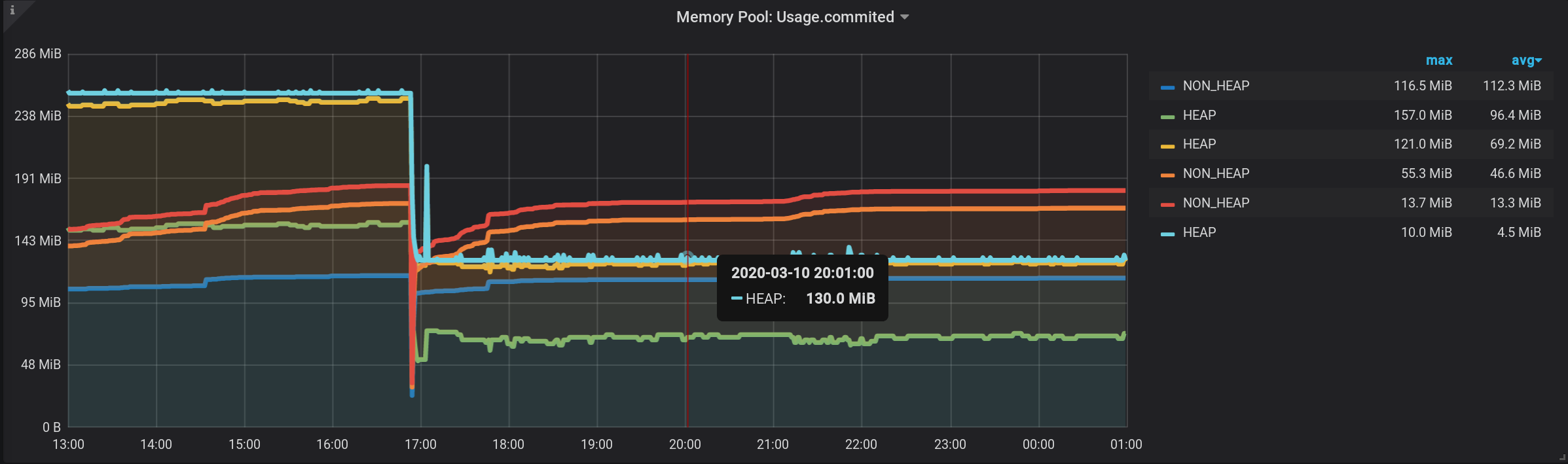
Remember the values for 20:00: NON_HEAP pools 172.5 MiB , and HEAP pools 128 MiB . We will focus on these values in the future.
In the context of Type : name , we obtained the metric value easily.In the context of only the name tag , the metric value is also easy to obtain, since all the names of the memory pools are unique, and it is enough to leave the grouping of results only by name .The question remains: how to get what size is allocated for all HEAP pools and all NON_HEAP pools in total?
1. Just the amount grouped by Type tag
1.1. Sum grouped by tag
The first solution that may come to mind is to group the values by the Type tag and calculate the sum of the values in each group. Such a query will look like this: A textual representation of a sum calculation request grouped by Type tag with all Grafana variables :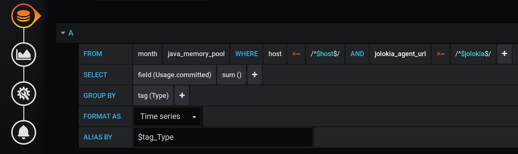
SELECT sum("Usage.committed")
FROM "telegraf"."month"."java_memory_pool"
WHERE
    host =~ /^${host:regex}$/ AND
    jolokia_agent_url =~ /^${jolokia:regex}$/ AND
    $timeFilter
GROUP BY
    "Type"
This is a valid query, but it will return only two points: the sum will be calculated with grouping only by the Type tag with two values (HEAP and NON_HEAP). We won’t even see the schedule. There will be two free-standing points with a huge sum in values (more than 3 TiB): Such a sum is not suitable, a breakdown into time intervals is needed.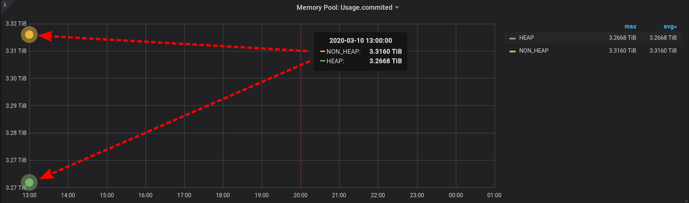
1.2. Amount grouped by tag per minute
In the original query, we grouped metrics by a custom $ granularity interval . Let's do the grouping now by a custom interval.This query will turn out, it added GROUP BY time($granularity): We get inflated values, instead of 172.5 MiB by NON_HEAP we see 4.88 GiB: Since metrics are sent to InfluxDB once every 2 seconds (see telegraf.conf above), the sum of readings in one minute will not give the amount in the moment, and the sum of thirty such amounts. We cannot divide the result by constant 30 either. Since $ granularity is a parameter, it can be set to both 1 minute and 10 minutes. And the value of the amount will change.
1.3. Tag grouped per second
In order to correctly get the metric value for the current metric collection intensity (2 seconds), you need to calculate the amount for a fixed interval that does not exceed the metric collection intensity.Let's try to display statistics with a grouping in seconds. Add to the GROUP BYgrouping time(1s): With such a small granularity, we get a huge number of points for our time interval of 12 hours (12 hours * 60 minutes * 60 seconds = 43,200 intervals, 43,201 points per line, the last of which is null): 43,201 points in each line of the graph. There are so many points that InfluxDB will form a response for a long time, Grafana will take a response longer, and then the browser will draw such a huge number of points for a long time.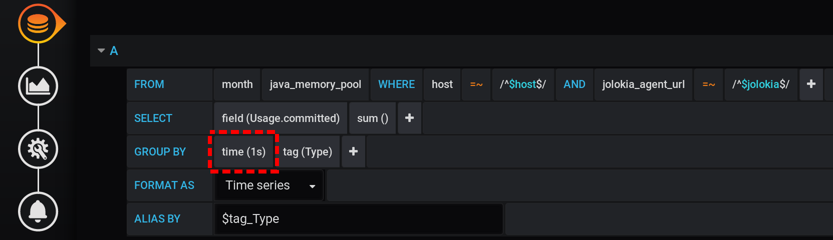
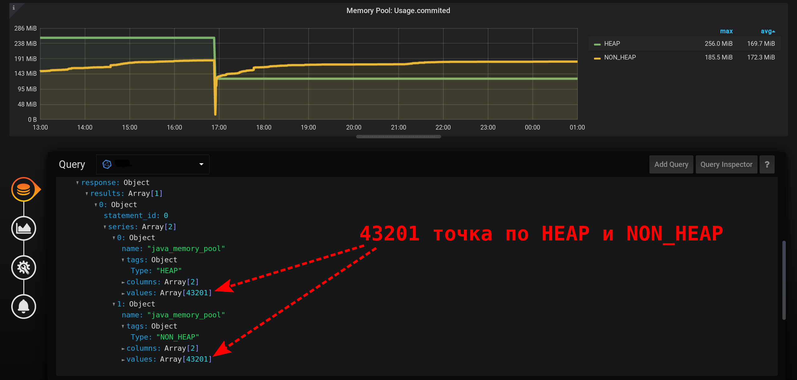 And not in every second there are points: metrics were collected every 2 seconds, and grouping by every second, which means that every second point will be null. To see a smooth line, configure the connection of non-empty values. Otherwise, we won’t see the graphs: Previously, Grafana was such that the browser hung during the drawing of a large number of points. Now the version of Grafana has the ability to draw several tens of thousands of points: the browser simply skips some of them, draws a graph using the thinned data. But the graph is smoothed out. Highs are displayed as average highs.
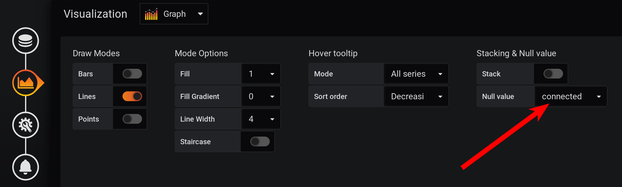 As a result, there is a graph, it is displayed accurately, the metrics at 20:00 are calculated correctly, the metrics in the chart legend are calculated correctly. But the graph is smoothed: bursts are not visible on it with an accuracy of 1 second. In particular, the HEAP surge at 17:03 disappeared from the chart, the HEAP chart is very smooth: The minus in performance will clearly manifest itself over a longer time interval. If you try to build a graph in a month (720 hours), and not in 12 hours, then everything will freeze with such a small granularity (1 second), there will be too many points. And there is a minus in the absence of peaks, a paradox - due to the high accuracy of obtaining metrics, we get a low accuracy of their display .
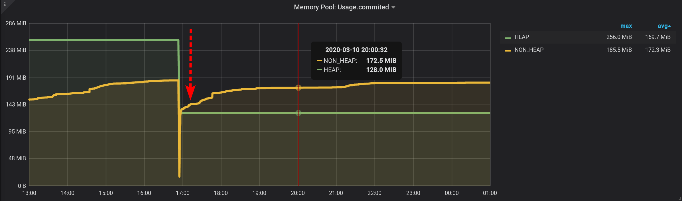
2. Grafana-way. We use a stack of values
It was not possible to create a simple and productive solution with InfluxDB and the Grafana query designer . We will only try using Grafana tools to summarize the metrics displayed in the original chart. And yes, this is possible!2.1. Just make Hover tooltip / Stacked value: cummulative
We will leave the request for choosing metrics unchanged, the same as in the section “How it all began”: Metrics will be grouped by Type and name . But we will only display the Type tag in the names of the graphs : And in the visualization settings, we will group the metrics by Grafana stacks : First, add the separation of two tags into two different stacks A and B, so that their values do not intersect: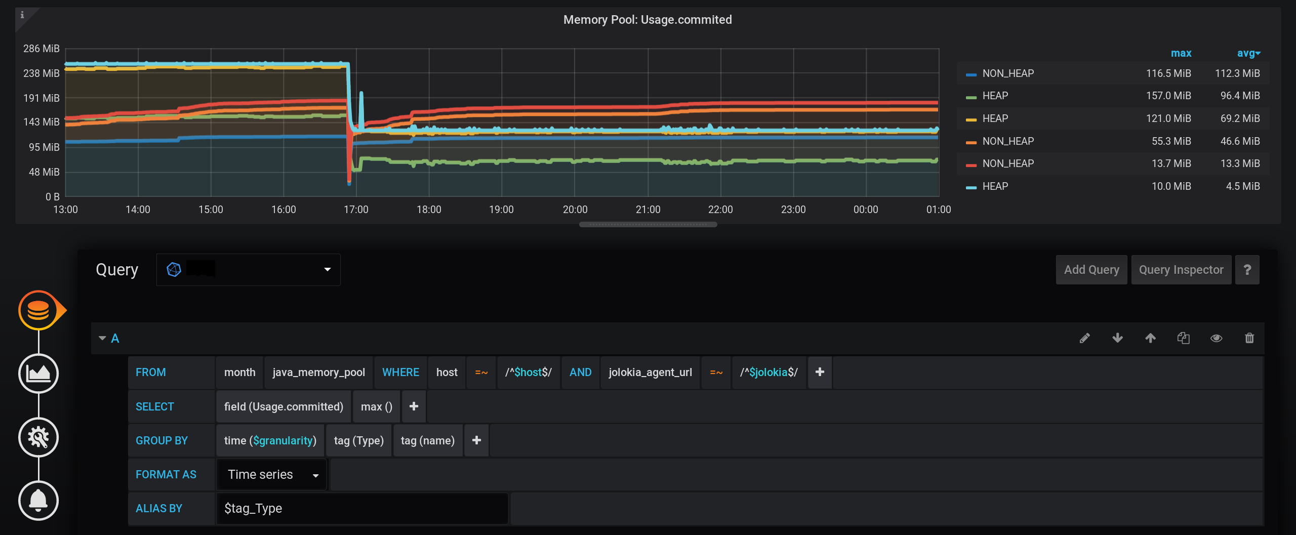
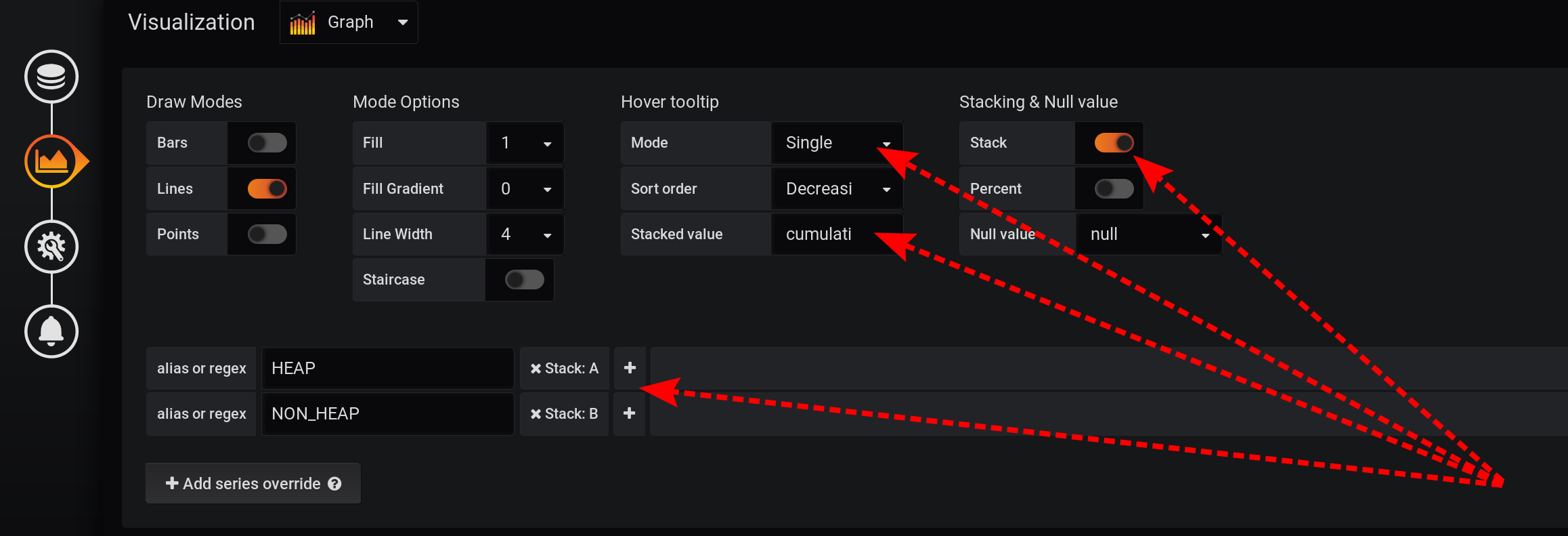
- Add series override / HEAP / Stack : A
- Add series override / NON_HEAP / Stack : B
Then configure the visualization of metrics to display the total values in a tooltip with graphs:- Stacking & Null value / Stack : On
- Hover tooltip / stacked value : cummulative
- Hover tooltip / mode : single
Due to the different features of Grafana, you need to perform actions in that order. If you change the order of actions or leave some fields with default settings, something will not work:- Stack A B Stacking & Null value / Stack: On, ;
- Hover tooltip / Mode , Single, Hover tooltip .
And now, we see many lines, such to ourselves. But! If you hover over the topmost NON_HEAP , the tooltip will show the sum of the values of all NON_HEAPs . The amount is considered true, already by Grafana means : And if you hover over the topmost chart with the name HEAP , we will see the amount by HEAP . The graph is displayed correctly. Even the HEAP surge at 17:03 is visible: Formally, the task is completed. But there are cons - a lot of extra charts are displayed. You need to get the cursor to the very top of them. And in the legend to the graph, not cumulative, but individual values are displayed, so the legend has become useless.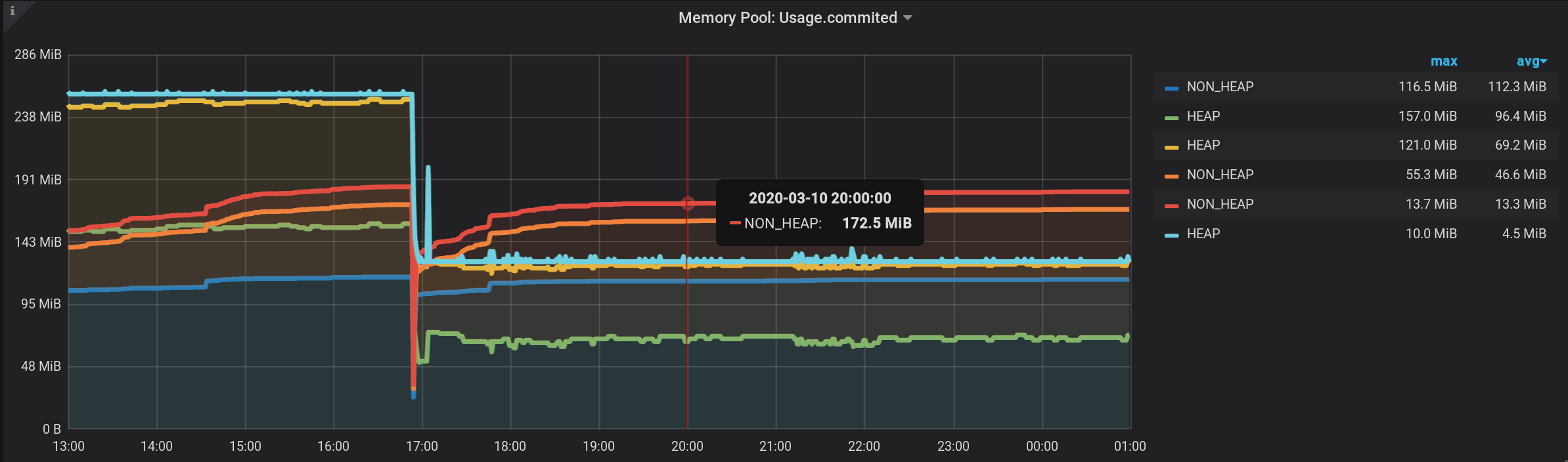
2.2. Stacked value: cummulative with hiding intermediate lines
Let's fix the first minus of the previous solution: make sure that extra charts are not displayed.For this:- Add new metrics with a different name and value 0 to the results.
- Add new metrics to Stack A and Stack B , to the top of the stack.
- Hide from the display - the original lines of HEAP and NON_HEAP .
We add two new ones after the main request: request B for receiving a series with values 0 and name [NON_HEAP] and request C for receiving a series with values 0 and name [HEAP] . To get 0, we take the first value of the “Usage.committed” field in each time group and subtract it: first (“Usage.committed”) - first (“Usage.committed”) - we get a stable 0. The names of the graphs are changed without losing meaning due to the square brackets: [NON_HEAP] and [HEAP] : [HEAP] and HEAP are combined into Stack A , and also hide all HEAP . [NON_HEAP]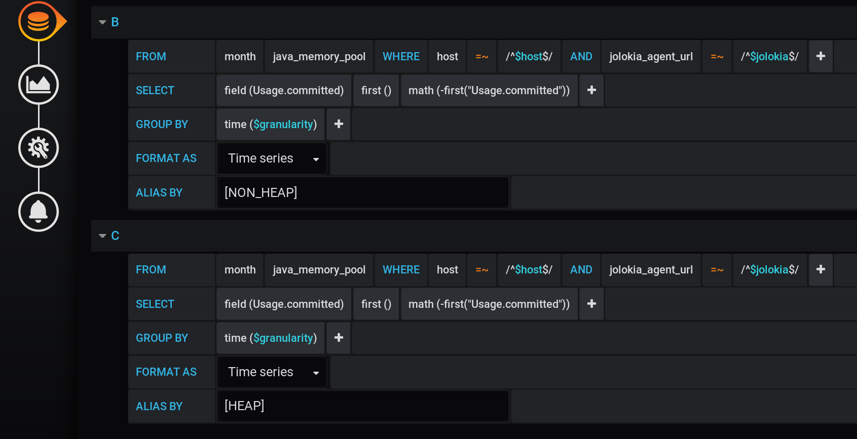 and combine NON_HEAP in Stack B and hide NON_HEAP : Get the
correct amount by [NON_HEAP] in the Tooltip when hovering over the chart: Get the correct amount by [HEAP] in the Tooltip when hovering over the chart. And even all the bursts are visible: And the schedule is formed quickly. But the legend always displays 0, the legend has become useless. Everything worked out! True bypass is through the Grafana stacks . It is because of this that the article was added to the Abnormal Programming category .
and combine NON_HEAP in Stack B and hide NON_HEAP : Get the
correct amount by [NON_HEAP] in the Tooltip when hovering over the chart: Get the correct amount by [HEAP] in the Tooltip when hovering over the chart. And even all the bursts are visible: And the schedule is formed quickly. But the legend always displays 0, the legend has become useless. Everything worked out! True bypass is through the Grafana stacks . It is because of this that the article was added to the Abnormal Programming category .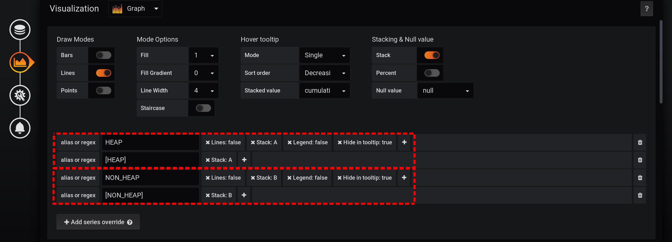


3. The sum of the highs with the subquery
Since we have already embarked on the path of abnormal programming with a bunch of Grafana and InfluxDB , let's continue. Let's make InfluxDB return a small number of points and make the legend appear.3.1 Sum of increments of the cumulative sum of maxima
Let's delve into the possibilities of InfluxDB . Previously, I often helped out by taking the derivative of the cumulative amount, so we’ll try to apply this approach now. Let's switch to the mode of manual editing of requests: Let's make such a request:
SELECT sum("U") FROM (
        SELECT non_negative_difference(cumulative_sum(max("Usage.committed"))) AS "U"
        FROM "month"."java_memory_pool"
        WHERE
            (
                "host" =~ /^${host:regex}$/ AND
                "jolokia_agent_url" =~ /^${jolokia:regex}$/
            ) AND
            $timeFilter
        GROUP BY time($granularity), "Type", "name"
)
GROUP BY "Type", time($granularity)
Here the maximum value of the metric in the group by time is taken and the sum of such values from the moment the reference begins, grouped by the Type and name tags . As a result, at each moment of time there will be a sum of all indications by type ( HEAP or NON_HEAP ) with separation by pool name, but not 30 values are summed, as was the case in version 1.2, but only one is the maximum.And if we take the non_negative_difference increment of such a cumulative sum for the last step, then we will get the sum value of all data pools grouped by Type and name tags at the beginning of the time interval.Now, to get the amount by tag onlyType , without grouping by name tag , you need to make a top-level request with similar grouping parameters, but without grouping by name .As a result of such a complex query, we get the sum of all types.Perfect schedule. The sum of the maxima is calculated correctly. There is a legend with the correct values, non-zero. In the tooltip you can display all the metrics, not just Single. Even HEAP bursts are displayed : One thing but - the request turned out to be difficult: the sum of the increment of the cumulative sum of maxima with a change in the grouping level.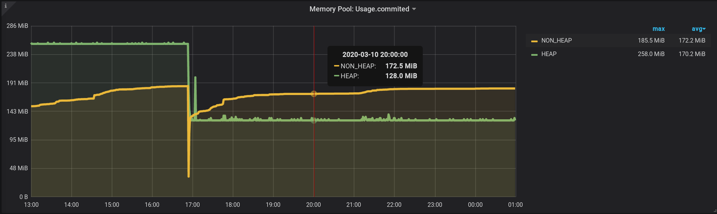
3.2 Sum of highs with a change in the grouping level
Can you do something simpler than in version 3.1? Pandora's box is already open, we switched to manual query editing mode.There is a suspicion that receiving an increment from the cumulative amount leads to a zero effect - one extinguishes the other. Get rid of non_negative_difference (cumulative_sum (...)) .Simplify the request.We simply leave the sum of the maxima, with a decrease in the grouping level:SELECT sum("A")
FROM (
SELECT max("Usage.committed") as "A"
FROM "month"."java_memory_pool"
WHERE
(
"host" =~ /^${host:regex}$/ AND
"jolokia_agent_url" =~ /^${jolokia:regex}$/
) AND
$timeFilter
GROUP BY time($granularity), "Type", "name"
)
WHERE $timeFilter
GROUP BY time($granularity), "Type"
This is a quick simple query that returns only 721 points per series in 12 hours, when grouped by minutes: 12 (hours) * 60 (minutes) = 720 intervals, 721 points (last empty). Please note that the time filter is duplicated. It is in the subquery and in the grouping request: Without $ timeFilter, in the external grouping request, the number of returned points will not be 721 in 12 hours, but more. Since the subquery is grouped for the interval from ... to , and the grouping of an external request without a filter will be for the interval from ... now . And if in Grafana a time interval not last X-hours is selected (not such that to = now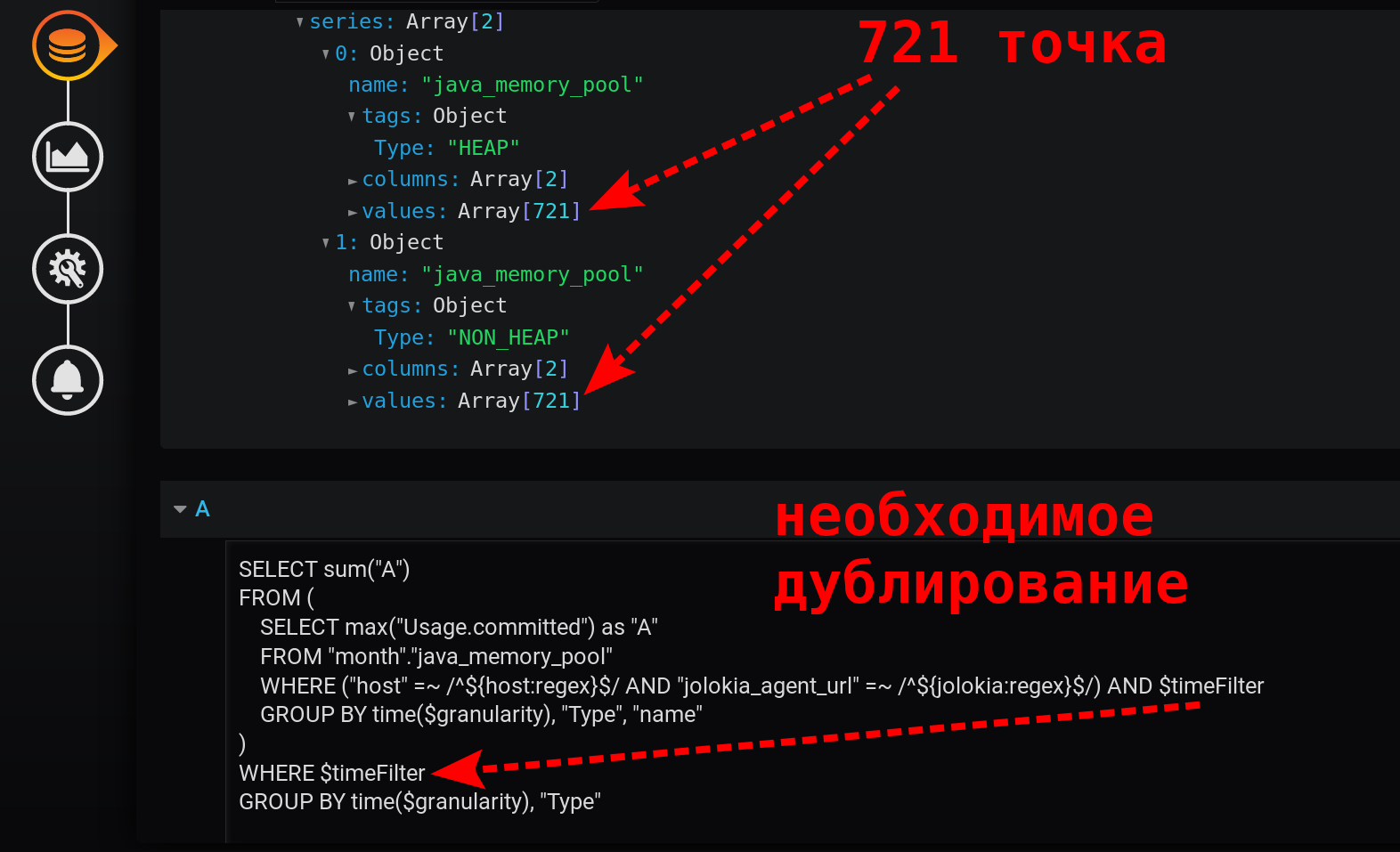 ), but for the interval from the past ( to < now ), then empty points with a null value at the end of the selection will appear.The resulting graph turned out to be simple, fast, correct. With a legend that displays summary metrics. With tooltip for multiple lines at once. And also with the display of all bursts of values: The result is achieved!
References (instead of references)
Distributions of the tools used in the article:Documentation about the capabilities of the tools used in the article:The combination of Grafana and InfluxDB needs to be well known to performance testing engineers. And in this bundle, many simple tasks are very interesting, and they can not always be solved by normal programming methods.Sometimes abnormal programming skills may be needed with the Grafana features and subtleties of the InfluxDB query language .In the article, four steps were taken into account of the implementation of summarizing a metric with a grouping by one tag, but which has several tags. The task was interesting. And there are many such tasks.I am preparing a report on the subtleties of programming with Grafana and InfluxDB. I will periodically publish materials on this topic. In the meantime, I will be happy with your questions on the current article.