Faraday law or how a magnet gets stuck in a copper pipe

Image taken from the Popular Mechanics website .

Many have seen the experience with a permanent magnet, which seems to get stuck inside a thick-walled copper tube. In this article we will understand the physics of the process.
First, we write the formula of the magnetic field of the permanent magnet, and calculate which magnetic flux passes through the cross section of the pipe, then make the magnet move and find out what induced electric current arises in the metal, what is the dissipated electric power, write and solve the equation of motion of the permanent magnet.

And if you read up to this place and were not afraid, welcome to kat - then it will be more interesting!

I myself have been thinking for a long time to thoroughly understand this issue. And recently, a conversation with a work colleague started. His child was asked to make a scientific demonstration at school, for which dad got a piece of a copper pipe and a neodymium-iron-boron magnet. The child understood, made a demonstration of experience in front of the class, gave explanations, but neither the class nor the teacher were particularly impressed. At a competition of scientific experiments, a volcano (!) From soda and citric acid won =) My colleague and I took a quick look and realized that it was clear, that it was dark. And in the literature not much has been written on this topic. This conversation and motivated me to try to get through the jungle. In this article I write what I did.

Experiment description

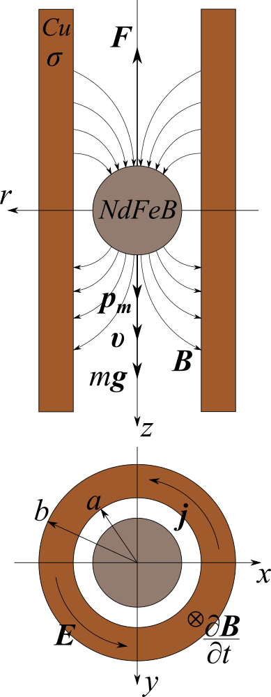
Let's start by watching a video demonstrating the experience. Before delving into the theory, it will be useful to present a picture of what is happening in general. On the Internet, this experience has been explained and demonstrated on video many times. But I also need to describe it here, so that later it is clear what we are repelling from.

The experimenter places a permanent magnet in the form of a small ball in a copper pipe, which he holds vertically. Contrary to expectations, the ball does not fall through the pipe with an acceleration of gravity, but moves inside the pipe much more slowly.

So, in experience we observe how a permanent magnet moves inside a hollow copper pipe at a constant speed. We fix an arbitrary point in the body of the copper tube and mentally draw a cross section. A magnetic flux generated by a permanent magnet passes through this section of the copper pipe. Due to the fact that the magnet moves along the pipe, a variablemagnetic flux, either increasing or decreasing depending on whether the magnet is approaching or moving away from the point where we mentally conducted the section. According to Maxwell's equations, an alternating magnetic flux generates a vortex electric field, generally speaking, in the whole space. However, only where there is a conductor, does this electric field set in motion free charges located in the conductor - does a circular electric current arise, which already creates its own magnetic field and interacts with the magnetic field of a moving permanent magnet. Simply put, a circular electric current creates a magnetic field of the same sign as a permanent magnet, and a certain dissipative force acts on the magnet, and in particular the friction force. The reader can rightly ask a question:"Friction of what about what?" Friction occurs between the magnetic field of the dipole and the conductor. Yes, this friction is not mechanical. Rather, the bodies do not touch. Well, let! There is still friction!

In general, in words everything looks more or less complex, but can this be described in the language of mathematics? Let's get started ...

Mathematical description

First things first, we need a mathematical model of a permanent magnet. In my opinion, it will be convenient to imagine a permanent magnet as a magnetic dipole.

$$

$$\vec{B}=\frac{\mu_0}{4\pi}\left(\frac{3(\vec{p}_m\cdot\vec{r})\vec{r}}{r^5}-\frac{\vec{p}_m}{r^3}\right)$$

The notation is accepted here. $$$\vec{r}=(r,z)$ Is the radius vector from the center of the dipole to the observation point, $$$\vec{p}_m$Is the vector of the dipole moment.

Next, we need to write$$$z$- a component of the magnetic induction vector for calculating the magnetic flux captured in the cross section of the metal of the copper pipe. We write$$$z$-component of the magnetic field here

$$

$$B_z(r,z) = \frac{\mu_0\,p_m}{4\pi}\frac{2z^2 - r^2}{\left(r^2 + z^2\right)^\frac{5}{2}}$$

Now we write the expression for the magnetic flux through the area covered by a circle of radius $$$r$ on distance $$$z$ from the dipole.

$$

$$\Phi(r,z) = \int_0^{2\pi}\int_0^r B_z(r',z)\,r'\,dr'\,d\varphi = 2\pi\int_0^r \frac{\mu_0\,p_m}{4\pi}\frac{2z^2 - r'^2}{\left(r'^2 + z^2\right)^\frac{5}{2}}\,r'\,dr'$$

You will not believe it, but this integral is taken. I will not bore. The answer is very beautiful

$$

$$\Phi(r,z) = \frac{\mu_0\,p_m}{2}\frac{r^2}{\left(r^2 + z^2\right)^\frac{3}{2}}$$

Due to the fact that the dipole moves along the axis $$$z$ with speed $$$v$, you must also do a standard lookup $$$\Phi(r, z)\rightarrow \Phi(r, z - v t)$
It seems that it’s time to call for help one of Maxwell’s great equations, namely, the very equation that describes Faraday’s law :

Change in magnetic flux passing through an open surface $$$S$taken with the opposite sign is proportional to the circulation of the electric field in a closed loop $$$L$which is the boundary of the surface $$$S$

$$

$$\oint_L \vec{E}\,dl = -\frac{\partial}{\partial t}\int_S \vec{B}\,d\vec{s}$$

Or, the same thing

$$

$$2\pi r E_\varphi = -\frac{\partial}{\partial t}\Phi(r,z - v t)$$

Here we used the axial symmetry of the problem with respect to the axis $$$z$, and also took into account that the induced electric field has only the azimuthal component $$$\vec{E} = E_\varphi \vec{e}_\varphi$.
From here one can find the azimuthal component of the electric field induced by the magnet.

$$

$$E_\varphi(r,z) = -\frac{1}{2\pi r}\frac{\partial}{\partial t}\Phi(r, z - v t)=-\frac{3\mu_0\,p_m}{4\pi}\frac{rv(z-v t)}{\left(r^2 + (z-v t)^2\right)^\frac{5}{2}}$$

Now that we have an expression for the electric field, we can recall the pipe. As shown in the figure above, the inner radius of the pipe is$$$a$and the external - $$$b$. The pipe material is copper. At the moment, we will only need the electrical conductivity of copper. We denote the conductivity by$$$\sigma$.
An electric field inside a conductor causes an electric current. Therefore, we can write Ohm's law in differential form

$$

$$\vec{j} = \sigma \vec{E}$$

Electric current, in turn, causes ohmic losses inside the conductor. In other words, energy is dissipated inside the conductor and goes into the form of heat, strictly speaking, in our case, in the entire volume of the conductor.
The volume power density of ohmic losses is by definition equal to

$$

$$w = \vec{j}\cdot\vec{E} = \sigma E^2$$

On the other hand, when the magnet moves from top to bottom, the potential energy of the magnet in the Earth’s gravitational field decreases, however, the speed of motion remains constant, that is, does not increase , as it happens with free fall. This means only one thing: the potential energy of the magnet is dissipated inside the conductor. And from the point of view of the forces acting on the magnet, the friction force acts on it, which slows it down and dissipates the potential energy of the magnet into heat.
We now write the power balance in the problem: the rate of decrease of potential energy is equal to the power of ohmic losses in the conductor.

$$

$$\frac{dE_p}{dt} = P$$

$$

$$-mg\dot{z} = \int_V w\,dV$$

$$

$$mgv = \int_{-\infty}^{\infty}\int_0^{2\pi}\int_a^b \sigma E^2\,r\,dr\,d\varphi\,dz$$

It should be noted here that the potential energy in the coordinates shown in the figure above will be equal to $$$E_p = - mgz$, and to find the total power of ohmic losses, it is necessary to integrate $$$w$over the entire volume of the conductor. We consider the pipe length to be infinite. This is not so far from the truth, given that in the experiment from the video, the diameter of the magnet is much smaller than the length of the pipe.

The last triple integral looks very complicated. And so it is! But, firstly, azimuthal integration$$$\varphi$ can be replaced simply by multiplying by $$$2\pi$due to the axial symmetry of the problem. Secondly, the integration order in this particular integral can be changed and first integrated over$$$z$and then after $$$r$. Thirdly, when integrating over$$$z$ over infinite limits, we can safely discard the term $$$-vt$. The remaining integral is taken by the machine.

$$

$$\int_{-\infty}^\infty \frac{z^2\,dz}{\left(r^2 + z^2\right)^5} = \frac{5\pi}{128r^7}$$

The result is an answer for the full power of ohmic losses

$$

$$P = \frac{15}{1024}\,\mu_0^2\,p_m^2\,\sigma\left(\frac{1}{a^3} - \frac{1}{b^3}\right)v^2 = k\,v^2$$

Here, after the second equal sign, we designated the coefficient of friction

$$

$$k = \frac{15}{1024}\,\mu_0^2\,p_m^2\,\sigma\left(\frac{1}{a^3} - \frac{1}{b^3}\right)$$

Note that the coefficient of friction $$$k$ depends only on the magnetization of the magnet $$$p_m$, conductor material properties $$$\sigma$ and geometric dimensions of the pipe $$$a$ and $$$b$- that is, it depends solely on the parameters of the magnet and the pipe and does not depend, for example, on speed or time. This is a good sign for us and a small credit for the found formulas! From here it becomes clear why a copper pipe was chosen for demonstration of experience, and not, say, a steel pipe. Friction linearly depends on conductivity$$$\sigma$, and the conductivity of steel is less by an order of magnitude.



Can now record

$$

$$mgv=kv^2\\mg = kv$$

And suddenly (!), Before us is Newton’s third law! The strength of the action is equal to the strength of the reaction. We can find the steady speed of the magnet

$$

$$v_s = \frac{mg}{k}$$

Equation of motion

It was the turn of the equation of motion. Using Newton’s second law, it will be written very simply

$$

$$ma=mg - kv\\ m\ddot{z} + k\dot{z} = mg$$

Solve the equation for $$$z(t)$uninteresting, because well, just the coordinate changes at a constant speed. It is much more useful to know how quickly the fall stabilizes, which equals the steady-state fall rate. In general, you need to solve this equation for speed

$$

$$\dot{v} + \frac{k}{m} v = g$$

And the solution will be

$$

$$v(t) = v_0\,e^{-\alpha t} + v_s\left(1 - e^{-\alpha t}\right)$$

Here $$$\alpha = k/m$- attenuation coefficient. The characteristic time to reach the steady fall mode is$$$\tau = \alpha^{-1}$. Starting speed -$$$v_0$, steady speed - $$$v_s$.

In general, this is the equation of a skydiver. This is probably why the article of Popular Mechanics is called “Magnetic Parachute”.

Numerical experiment

And now there will be something for which all this was conceived. You brought a theory here, you know. What is she capable of? Suddenly it's just like a shadow on the wattle fence? Or it doesn’t work at all ...

First you need to deal with the geometry of the problem. The video from MIT, therefore, is American. I'll try to guess the size of their demo installation in inches (they also like to measure everything in inches). The size of the magnet is similar to$$$d = 1/2$inches in diameter. This is one of those that are on sale. Then the mass of such a magnet will be approximately$$$m = 8$ d. The length of the copper pipe is similar to $$$l = 12$ inches (1 ft), and the inner and outer diameters of the pipe are most likely $$$2a = 3/4$ inches $$$2b = 3/2$inches.

With geometry, sort of sorted out. Now physical properties. Copper conductivity$$$59.5\times 10^6$S / m

Earlier it was written here that I could not link the residual magnetization of a neodymium magnet with its equivalent magnetic moment. But there were good people in the comments. UserDenishwthe source suggested (see paragraph 5 in the list of references) where you can read, helped make the necessary calculations, and even checked them on the FEMM simulator.


Calculation of the magnetic field of a ball from NdFeB on the FEMM simulator. Image provided by userDenishw

So, what was found out. NdFeB magnet belongs to the class of paramagnets, because under the influence of an external field, the internal field is amplified. Moreover, the NdFeB alloy is able to maintain the internal field after the termination of the external field. This fact classifies NdFeB as a ferromagnet. If we denote the induction of the internal field of a magnet by$$$B$, and the external magnetic field $$$H$then equality

$$

$$B = \mu \mu_0 H = (1 + \chi)\mu_0 H = \mu_0(H + I)$$

Here $$$\chi$ - the magnetic susceptibility of the substance, and $$$I$Is the magnetization vector of the substance.

When a magnet is made in a factory, it is magnetized by an external field.$$$H$and then the external field is turned off, and the magnet retains some residual magnetization $$$B_r$. It is known that for neodymium magnets, the remanent magnetization is approximately$$$B_r = 1\,..\,1.3$ T. Now, if you exclude the external field $$$H$ from the previous equation, we get

$$

$$B_r = \mu_0I$$

Where do we find the magnetic moment per unit volume of material $$$I$ as

$$

$$I = \frac{B_r}{\mu_0}$$

To find the magnetic moment of the magnet as a whole, you need to multiply $$$I$ per ball volume $$$V$

$$

$$p_m=IV=I\cdot\frac{4}{3}\pi\left(\frac{d}{2}\right)^3$$

For residual magnetization $$$B_r = 1$ T is obtained $$$p_m = 0.853$Am².
Below is a graph$$$z$- components of the magnetic field depending on the radial coordinate in our problem at a distance of half the diameter of the ball.


$$$z$-component of a magnetic field near the surface of a permanent magnet

Once it was possible to measure with a device. Fields directly on the surface of such magnets are usually less than the residual magnetization and amount to about several thousand gauss. What I measured for a rectangular magnet was about 4,500 Gs. Therefore, we have a very realistic result on the magnetic field plot.

Now we will use the solution of the equation of motion to plot the speed of the magnet. For all the parameters selected above, the friction coefficient is equal to$$$k = 1.015$ N / (m / s), steady speed - $$$v_s = 7.77$cm / s - just about 3 inches per second! In the video, the ball passes through a 12-inch pipe in about 4 seconds.


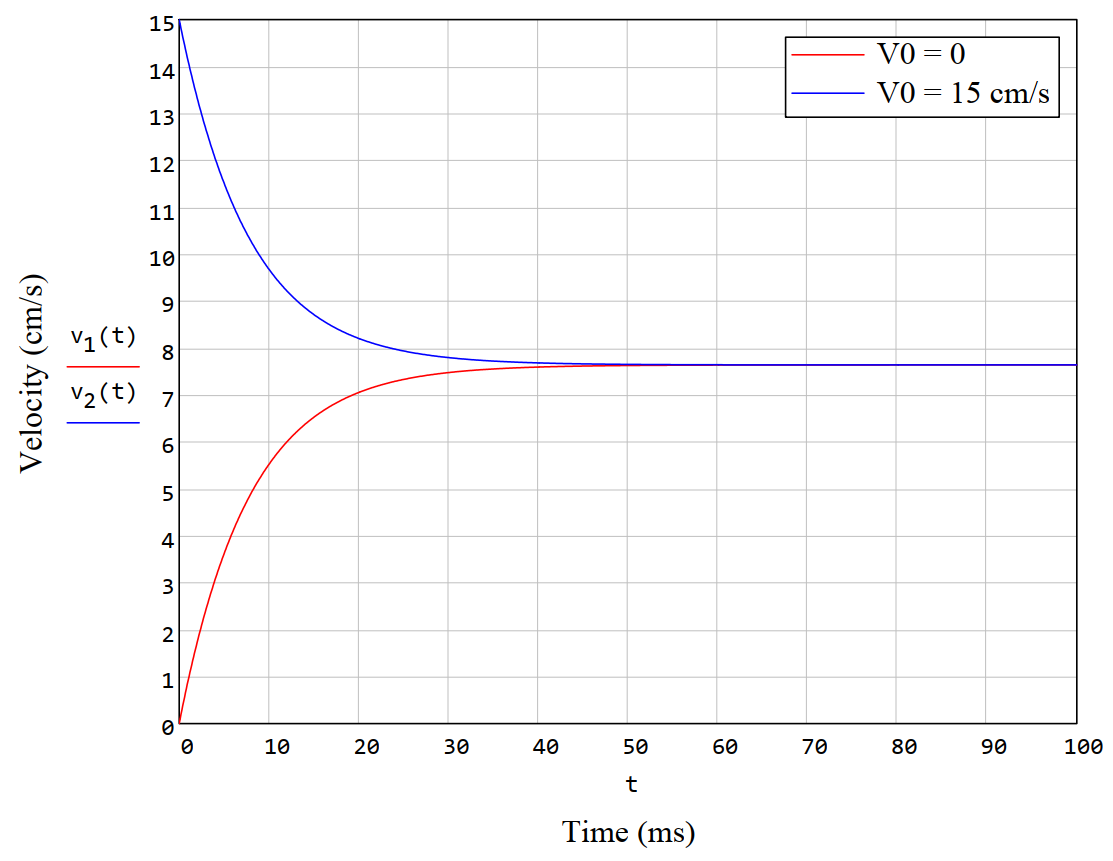Graph for solving the equation of motion of a magnet in a copper pipe


And we continue. Power dissipation is approximately$$$P \approx 6$ mW, and the characteristic time for reaching the steady state is $$$\tau \approx 8$ms Below are the graphs.$$$v(t)$ for two different initial speeds: zero, and $$$v_0 = 15$cm / s.

And in addition, the uservashu1rightly remarked that it would be nice to know the current induced in a copper pipe. Well, and it is possible. Integrate

$$

$$J = \int_{0}^{\infty}\int_a^b \sigma E(r,z)\,dr\, dz = \frac{\sigma\, v\,\mu_0\, p_m}{4\pi}\left(\frac{1}{a} - \frac{1}{b}\right)$$

Integrate by $$$z$it is necessary according to semi-infinite limits, since in the other half of the pipe the current flows in the opposite direction. I got the answer$$$J = 20$A. Honestly, I did not expect to get such a big current. At the uservashu1it turned out 50 A, which, apparently, is also not far from reality. I thinkvashu1I calculated the sum of the currents in the entire pipe, which, for reasons of power, is also reasonable.

Here is such a study. Hope that was interesting. Leave your comments. I will try to answer everyone. If you liked the article, support the author like or plus in karma. Thanks for reading.

Literature

1. Jackson, J. Classical electrodynamics: Per. from English World, 1965.
2. Landau, L.D., & Lifshitz, E.M. (1941). Field theory. Moscow; Leningrad: State Publishing House of technical and theoretical literature.
3. Sivukhin, D. V. “General course of physics. Volume 3. Electricity. " Moscow, publishing house "Science", the main edition of the physical and mathematical literature (1977).
4. Yavorsky, B. M., and A. A. Detlaf. "Handbook of Physics." (1990).
5. Kirichenko N.A. Electricity and magnetism. Tutorial. - M .: MIPT, 2011 .-- 420 p.