🤛🏻 🙏🏾 ⚛️ Python News Bitcoin Price Prediction 🎑 🥡 👩‍🎓

A translation of the article was prepared ahead of the start of the Machine Learning course from OTUS.

Task

In this guide, we use the Bitcoin vs USD dataset .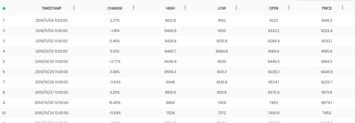

The above dataset contains a daily price summary, where the CHANGE column is the change in price as a percentage of the previous day's price ( PRICE ) versus new ( OPEN ).

Goal: To simplify the task, we will focus on predicting whether the price will rise ( CHANGE> 0 ) or fall ( CHANGE <0 ) the next day. (So we can potentially use predictions "in real life").

Requirements

Python 2.6+ or 3.1+ must be installed on the system
Install pandas , sklearn and openblender (using pip)

$ pip install pandas OpenBlender scikit-learn

Step 1. Get Bitcoin Data

To get started, let's import the necessary libraries:

import OpenBlender
import pandas as pd
import json

Now pull the data through the OpenBlender API .
First, let's define the parameters (in our case, this is just the id of the bitcoin dataset ):

# It only contains the id, we'll add more parameters later.
parameters = { 
 'id_dataset':'5d4c3af79516290b01c83f51'
}

Note: you will need to create an account on openblender.io (it’s free) and add a token (you will find it in the “Account” tab):

parameters = {     
   'token':'your_token',
   'id_dataset':'5d4c3af79516290b01c83f51'
}

Now let's put the data in the Dataframe 'df' :

# This function pulls the data and orders by timestamp
def pullObservationsToDF(parameters):
    action = 'API_getObservationsFromDataset'
    df = pd.read_json(json.dumps(OpenBlender.call(action,parameters)['sample']), convert_dates=False,convert_axes=False) .sort_values('timestamp', ascending=False)
    df.reset_index(drop=True, inplace=True)
    return df
df = pullObservationsToDF(parameters)

And look at them:

Note: the values may vary, as the dataset is updated daily !

Step 2. Data Preparation

To begin with, we need to create a forecasting target, which will be whether “ CHANGE ” will increase or decrease. To do this, add 'success_thr_over': 0 to the target threshold parameters:

parameters = {
   'token':'your_token',   
   'id_dataset':'5d4c3af79516290b01c83f51',
   'target_threshold':{'feature':'change', 'success_thr_over': 0}
}

If we pull the data from the API again:

df = pullObservationsToDF(parameters)
df.head()

The attribute “CHANGE” has been replaced by a new attribute 'change_over_0', which becomes 1 if “CHANGE” is positive and 0 if not. This will be a machine learning target.

If we want to predict the observation for "tomorrow", we will not be able to use the information from tomorrow, so let's add a delay of one period.

parameters = { 
   'token':'your_token',
   'id_dataset':'5d4c3af79516290b01c83f51',
   'target_threshold':{'feature':'change','success_thr_over' : 0},
   'lag_target_feature':{'feature':'change_over_0', 'periods' : 1}
}
df = pullObservationsToDF(parameters)
df.head()

This simply aligns 'change_over_0' with the data for the previous day (period) and changes its name to 'TARGET_change_over_0' .

Let's look at the dependency:

target_variable = 'TARGET_change_over_0'
df = df.dropna()
df.corr()[target_variable].sort_values()

They are linearly independent and unlikely to be useful.

Step 3. Get Business News Data

After searching for dependencies in OpenBlender , I found the Fox Business News dataset that will help generate good forecasts for our target.

We need to find a way to convert the values of the 'title' column to numerical characteristics, counting the repetitions of words and groups of words in the news summary, and compare them in time with our bitcoin dataset. It is easier than it sounds.

First you need to create a TextVectorizer for the 'title' attribute of the news:

action = 'API_createTextVectorizer'
vectorizer_parameters = {
    'token' : 'your_token',
    'name' : 'Fox Business TextVectorizer',
    'sources':[{'id_dataset' : '5d571f9e9516293a12ad4f6d',
                'features' : ['title']}],
    'ngram_range' : {'min' : 1, 'max' : 2},
    'language' : 'en',
    'remove_stop_words' : 'on',
    'min_count_limit' : 2
}

We will create a vectorizer to get all the signs as token words in the form of numbers. Above, we indicated the following:

name : let's call it 'Fox Business TextVectorizer' ;
anchor : id of the dataset and the names of signs that we will need to use as a source (in our case, only the 'title' column );
ngram_range : minimum and maximum length of a set of words for tokenization;
language : English
remove_stop_words : to remove stop words from the source;
min_count_limit : the minimum number of repetitions to be considered as a token (single occurrences are rarely useful).

Now run this:

res = OpenBlender.call(action, vectorizer_parameters)
res

Answer:

{  
    'message' : 'TextVectorizer created successfully.'
    'id_textVectorizer' : '5dc1a404951629331f6359dd',
    'num_ngrams': 4270
}

TextVectorizer was created , which generated 4270 n-grams according to our configuration. A little later we will need the generated id:

5dc1a404951629331f6359dd

Step 4. Compatible news summary with bitcoin dataset

Now we need to compare the news summary and the bitcoin exchange rate data in time. In general, this means that you need to combine two sets of data using a timestamp as a key. Let's add the combined data to our original data extraction options:

parameters = { 
   'token':'your_token',  
   'id_dataset':'5d4c3af79516290b01c83f51',
   'target_threshold' : {'feature':'change','success_thr_over':0},
   'lag_target_feature' : {'feature':'change_over_0', 'periods':1},
   'blends':[{'id_blend':'5dc1a404951629331f6359dd',
               'blend_type' : 'text_ts',
               'restriction' : 'predictive', 
               'specifications':{'time_interval_size' : 3600*12 }}]
}

Above, we indicated the following:

id_blend : id of our textVectorizer;
blend_type : 'text_ts' so that Python understands that it is a mixture of text and timestamp;
restriction : 'predictive' , so that there is no “mixing” of news from the future with all the observations, but only with those that were published earlier than the specified time.
blend_class : 'closest_observation' , so that only the closest observations are "mixed";
specifications : the maximum possible amount of elapsed time for transferring the observation, in this case 12 hours (3600 * 12). This means that every observation of the price of bitcoin will be predicted based on the news of the last 12 hours.

Finally, we just add a filter by the date 'date_filter' date , starting on August 20, because that's when Fox News started collecting data, and 'drop_non_numeric' so that we get only numbers:

parameters = { 
   'token':'your_token',
   'id_dataset':'5d4c3af79516290b01c83f51',
   'target_threshold' : {'feature':'change','success_thr_over':0},
   'lag_target_feature' : {'feature':'change_over_0', 'periods':1},
   'blends':[{'id_blend':'5dc1a404951629331f6359dd',
               'blend_type' : 'text_ts',
               'restriction' : 'predictive',
               'blend_class' : 'closest_observation', 
               'specifications':{'time_interval_size' : 3600*12 }}],
   'date_filter':{'start_date':'2019-08-20T16:59:35.825Z',
                   'end_date':'2019-11-04T17:59:35.825Z'},
   'drop_non_numeric' : 1
}

Note : I indicated November 4 as 'end_date' , since it was the day I wrote this code, you can change the date.

Let's get the data again:

df = pullObservationsToDF(parameters)
print(df.shape)
df.head()

(57, 2115)

Now we have more than 2000 signs with tokens and 57 observations.

Step 5. Apply ML to the prediction target

Now, finally, we have a clean dataset, and it looks exactly as we need it, with a time offset of the target and associated numerical data.

Let's look at the highest correlations with 'Target_change_over_0' :

Now we have some correlating attributes. Let's divide the dataset into training and test in chronological order so that we can train the model in early observations and test in later ones.

X = df.loc[:, df.columns != target_variable].values
y = df.loc[:,[target_variable]].values
div = int(round(len(X) * 0.29))
# We take the first observations as test and the last as train because the dataset is ordered by timestamp descending.
X_test = X[:div]
y_test = y[:div]
print(X_test.shape)
print(y_test.shape)
X_train = X[div:]
y_train = y[div:]
print(X_train.shape)
print(y_train.shape)

We have 40 observations for training and 17 for testing.
Now we import the necessary libraries:

from sklearn.ensemble import RandomForestRegressor
from sklearn.metrics import mean_squared_error
from sklearn.metrics import accuracy_score
from sklearn.metrics import roc_auc_score
from sklearn import metrics

Now, let's use a random forest (RandomForest) and make a prediction:

rf = RandomForestRegressor(n_estimators = 1000)
rf.fit(X_train, y_train)
y_pred = rf.predict(X_test)

To make it easier to understand, let's put the predictions and y_test in the Dataframe:

df_res = pd.DataFrame({'y_test':y_test[:,0], 'y_pred':y_pred})
df_res.head()

Our real 'y_test' is binary, but our forecasts are of type float , so let's round them up, assuming that if they are greater than 0.5, this means an increase in price, and if less than 0.5 - a decrease.

threshold = 0.5
preds = [1 if val > threshold else 0 for val in df_res['y_pred']]

Now, in order to better understand the results, we get the AUC, error matrix and accuracy indicator:

print(roc_auc_score(preds, df_res['y_test']))
print(metrics.confusion_matrix(preds, df_res['y_test']))
print(accuracy_score(preds, df_res['y_test']))

We got 64.7% of the correct predictions with 0.65 AUC.

9 times we predicted a decline, and the price decreased (right);
5 times we predicted a decrease, and the price increased (incorrectly);
1 time we predicted an increase, but the price decreased incorrectly);
2 times we predicted an increase, and the price increased (true).

Learn more about the course .