In this article, I will talk about a couple of simple tricks that are useful when working with data that does not fit in the local machine, but is still too small to be called Large. Following the English-language analogy (large but not big), we will call this data thick. We are talking about sizes of units and tens of gigabytes.[Disclaimer] If you love SQL, everything written below can cause you to have bright, most likely negative emotions, in the Netherlands there are 49262 Tesla, 427 of them are taxis, better not read further [/ Disclaimer]. The starting point was an article on the hub with a description of an interesting dataset - a complete list of vehicles registered in the Netherlands, 14 million lines, everything from truck tractors to electric bicycles at speeds above 25 km / h.The set is interesting, takes 7 GB, you can download it on the website of the responsible organization.The attempt to drive the data as it is in the pandas to filter and clean it ended in a fiasco (gentlemen of the SQL hussars, I warned!). Pandas fell from a lack of memory on the desktop with 8 GB. With a little bloodshed, the question can be resolved if you recall that the pandas can read csv files in pieces of moderate size. The fragment size in rows is determined by the chunksize parameter.To illustrate the work, we will write a simple function that makes a request and determines how many Tesla cars are in total and what proportion of them work in taxis. Without tricks with fragment reading, such a request first eats up all the memory, then it suffers for a long time, and at the end the ramp falls off.With fragment reading, our function will look something like this:
def pandas_chunky_query():
print('reading csv file with pandas in chunks')
filtered_chunk_list=[]
for chunk in pd.read_csv('C:\Open_data\RDW_full.CSV', chunksize=1E+6):
filtered_chunk=chunk[chunk['Merk'].isin(['TESLA MOTORS','TESLA'])]
filtered_chunk_list.append(filtered_chunk)
model_df = pd.concat(filtered_chunk_list)
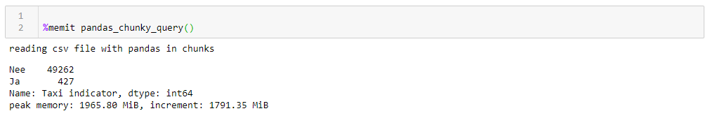
print(model_df['Taxi indicator'].value_counts())
By specifying a perfectly reasonable million lines, you can execute the query in 1:46 and using 1965 M of memory at its peak. All the numbers for a dumb desktop with something ancient, eight-core about 8 GB of memory and under the seventh Windows.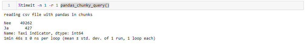
 If you change chunksize, then the peak memory consumption follows it quite literally, the execution time does not change much. For 0.5 M lines, the request takes 1:44 and 1063 MB, for 2M 1:53 and 3762 MB.The speed is not very pleasing, even less pleasing is that reading the file in fragments forces you to write adapted for this function, working with lists of fragments that must then be collected in a data frame. Also, the csv format itself is not very happy, which takes up a lot of space and is slowly read.Since we can drive data into a ramp, a much more compact Apachev format can be used for storageparquet where there is compression, and, thanks to the data scheme, it is much faster to read when it is read. And the ramp is quite able to work with him. Only now can not read them in fragments. What to do?- Let's have fun, take the Dask
 button accordion and speed up!Dask! A substitute for the ramp out of the box, able to read large files, able to work in parallel on several cores, and using lazy calculations. To my surprise about Dask on Habré there are only 4 publications .So, we take the dask, we drive the original csv into it and with minimal conversion, we drive it to the floor. When reading, dask swears at the ambiguity of data types in some columns, so we set them explicitly (for the sake of clarity, the same thing was done for the ramp, the operating time is higher taking into account this factor, the dictionary with dtypes is cut out for all the queries for clarity), the rest is for himself . Further, for verification, we make small improvements in the flooring, namely, we try to reduce the data types to the most compact ones, replace a pair of columns with text yes / no with Boolean ones, and convert other data to the most economical types (for the number of engine cylinders, uint8 is definitely enough). We save the optimized flooring separately and see what we get.The first thing that pleases when working with Dask is that we do not need to write anything superfluous simply because we have thick data. If you do not pay attention to the fact that the dask is imported, and not the ramp, everything looks the same as processing a file with a hundred lines in the ramp (plus a couple of decorative whistles for profiling).def dask_query():
print('reading CSV file with dask')
with ProgressBar(), ResourceProfiler(dt=0.25) as rprof:
raw_data=dd.read_csv('C:\Open_data\RDW_full.CSV')
model_df=raw_data[raw_data['Merk'].isin(['TESLA MOTORS','TESLA'])]
print(model_df['Taxi indicator'].value_counts().compute())
rprof.visualize()
Now compare the impact of the source file on performance when working with dasko. First we read the same csv file as when working with the ramp. The same about two minutes and two gigabytes of memory (1:38 2096 Mb). It would seem, was it worth it to kiss in the bushes? Now feed the board unoptimized parquet file. The request was processed in approximately 54 seconds, consuming 1388 MB of memory, and the file itself for the request is now 10 times smaller (about 700 MB). Here the bonuses are already visible convexly. CPU utilization of hundreds of percent is parallelization across several cores.
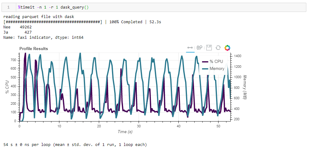 The previously optimized parquet with slightly altered data types in compressed form is only 1 Mb less, which means that without hints everything is compressed quite efficiently. The increase in productivity is also not particularly significant. The request takes the same 53 seconds and eats a little less memory - 1332 MB.Based on the results of our exercises, we can say the following:
- If your data is “fat” and you are used to a ramp - chunksize will help the ramp to digest this volume, the speed will be bearable.
- If you want to squeeze out more speed, save space during storage and you are not holding back using just a ramp, then dusk with parquet is a good combination.
Finally, about lazy computing. One of the features of the dask is that it uses lazy calculations, that is, calculations are not performed immediately as they are found in the code, but when they are really needed or when you explicitly requested it using the compute method. For example, in our function, dask does not read all the data into memory when we indicate to read the file. He reads them later, and only those columns that relate to the request.This is easily seen in the following example. We take a pre-filtered file in which we left only 12 columns from the initial 64, compressed parquet takes 203 MB. If you run our regular request on it, then it will execute in 8.8 seconds, and the peak memory usage will be about 300 MB, which corresponds to a tenth of the compressed file if you overtake it in a simple csv.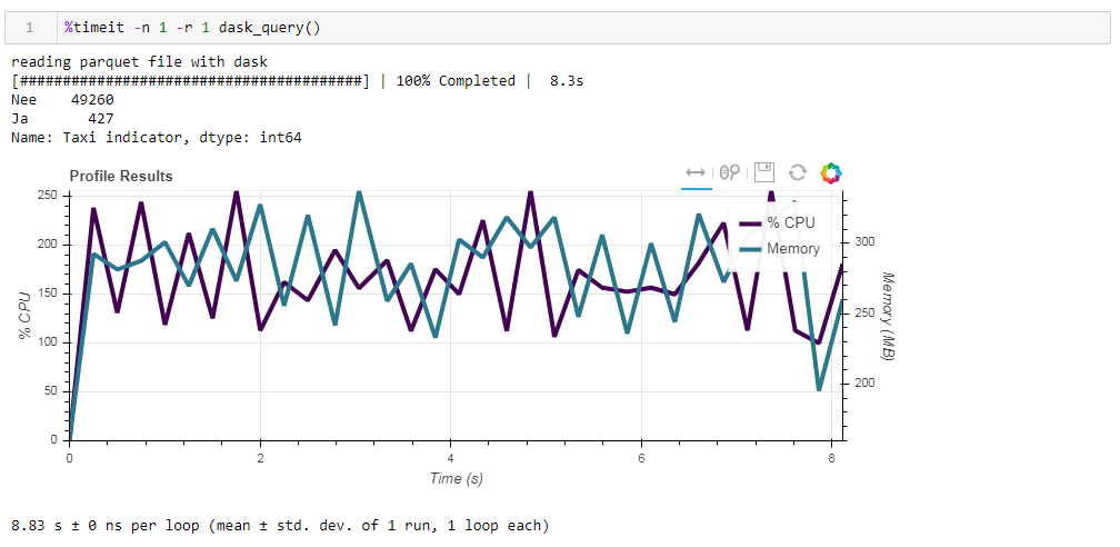 If we explicitly require you to read the file, and then execute the request, then the memory consumption will be almost 10 times more. We slightly modify our function by explicitly reading the file:
def dask_query():
print('reading parquet file with dask')
with ProgressBar(), ResourceProfiler(dt=0.25) as rprof:
raw_data=dd.read_parquet('C:\Open_data\RDW_filtered.parquet' ).compute()
model_df=raw_data[raw_data['Merk'].isin(['TESLA MOTORS','TESLA'])]
print(model_df['Taxi indicator'].value_counts())
rprof.visualize()
And here is what we get, 10.5 seconds and 3568 MB of memory (!)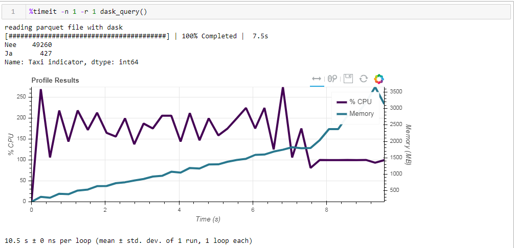 Once again we are convinced that the dask - it is competent to cope with its tasks itself, and once again climbing into it with micro-management does not make much sense.