Data processing and analysis specialists have many tools for creating classification models. One of the most popular and reliable methods for developing such models is to use the Random Forest (RF) algorithm. In order to try to improve the performance of a model built using the RF algorithm , you can use the optimization of the hyperparameter of the model ( Hyperparameter Tuning , HT). In addition, there is a widespread approach according to which the data, before being transferred to the model, is processed using the Principal Component Analysis , PCA). But is it worth it to use? Isn't the main purpose of the RF algorithm to help the analyst interpret the importance of the traits?Yes, the use of the PCA algorithm can lead to a slight complication of the interpretation of each “feature” in the analysis of the “importance of features” of the RF model. However, the PCA algorithm reduces the dimension of the feature space, which can lead to a decrease in the number of features that need to be processed by the RF model. Please note that the volume of calculations is one of the main disadvantages of the random forest algorithm (that is, it can take a long time to complete the model). Application of the PCA algorithm can be a very important part of modeling, especially in cases where they work with hundreds or even thousands of features. As a result, if the most important thing is to simply create the most effective model, and at the same time you can sacrifice the accuracy of determining the importance of the attributes, then the PCA may well be worth a try.Now to the point. We will be working with a breast cancer dataset - Scikit-learn “breast cancer” . We will create three models and compare their effectiveness. Namely, we are talking about the following models:
- The basic model based on the RF algorithm (we will abbreviate this RF model).
- The same model as No. 1, but one in which a reduction in the dimension of the feature space is applied using the principal component method (RF + PCA).
- The same model as No. 2, but built using hyperparameter optimization (RF + PCA + HT).
1. Import data
To get started, load the data and create a Pandas dataframe. Since we use a pre-cleared “toy” data set from Scikit-learn, then after that we can already start the modeling process. But even when using such data, it is recommended that you always start work by conducting a preliminary analysis of the data using the following commands applied to the data frame ( df):df.head() - to take a look at the new data frame and see if it looks as expected.df.info()- to find out the features of data types and column contents. It may be necessary to perform data type conversion before continuing.df.isna()- to make sure that there are no values in the data NaN. The corresponding values, if any, may need to be processed somehow, or, if necessary, it may be necessary to remove entire rows from the data frame.df.describe() - to find out the minimum, maximum, average values of the indicators in the columns, to find out the indicators of the mean square and probable deviation in the columns.
In our dataset, a column cancer(cancer) is the target variable whose value we want to predict using the model. 0means "no disease." 1- "the presence of the disease."import pandas as pd
from sklearn.datasets import load_breast_cancer
columns = ['mean radius', 'mean texture', 'mean perimeter', 'mean area', 'mean smoothness', 'mean compactness', 'mean concavity', 'mean concave points', 'mean symmetry', 'mean fractal dimension', 'radius error', 'texture error', 'perimeter error', 'area error', 'smoothness error', 'compactness error', 'concavity error', 'concave points error', 'symmetry error', 'fractal dimension error', 'worst radius', 'worst texture', 'worst perimeter', 'worst area', 'worst smoothness', 'worst compactness', 'worst concavity', 'worst concave points', 'worst symmetry', 'worst fractal dimension']
dataset = load_breast_cancer()
data = pd.DataFrame(dataset['data'], columns=columns)
data['cancer'] = dataset['target']
display(data.head())
display(data.info())
display(data.isna().sum())
display(data.describe())
. . , cancer, , . 0 « ». 1 — « »2.
Now split the data using the Scikit-learn function train_test_split. We want to give the model as much training data as possible. However, we need to have enough data at our disposal to test the model. In general, we can say that, as the number of rows in the data set increases, so does the amount of data that can be considered educational.For example, if there are millions of lines, you can split the set by highlighting 90% of the lines for training data and 10% for test data. But the test data set contains only 569 rows. And this is not so much for training and testing the model. As a result, in order to be fair in relation to the training and verification data, we will divide the set into two equal parts - 50% - training data and 50% - verification data. We installstratify=y to ensure that both the training and test data sets have the same ratio of 0 and 1 as the original data set.from sklearn.model_selection import train_test_split
X = data.drop('cancer', axis=1)
y = data['cancer']
X_train, X_test, y_train, y_test = train_test_split(X, y, test_size=0.50, random_state = 2020, stratify=y)
3. Data scaling
Before proceeding to modeling, you need to “center” and “standardize” the data by scaling it . Scaling is performed due to the fact that different quantities are expressed in different units. This procedure allows you to organize a “fair fight” between the signs in determining their importance. In addition, we convert y_trainfrom the Pandas data type Seriesto the NumPy array so that later the model can work with the corresponding targets.import numpy as np
from sklearn.preprocessing import StandardScaler
ss = StandardScaler()
X_train_scaled = ss.fit_transform(X_train)
X_test_scaled = ss.transform(X_test)
y_train = np.array(y_train)
4. Training of the basic model (model No. 1, RF)
Now create model number 1. In it, we recall that only the Random Forest algorithm is used. It uses all the features and is configured using the default values (details about these settings can be found in the documentation for sklearn.ensemble.RandomForestClassifier ). Initialize the model. After that, we will train her on scaled data. The accuracy of the model can be measured on the training data:from sklearn.ensemble import RandomForestClassifier
from sklearn.metrics import recall_score
rfc = RandomForestClassifier()
rfc.fit(X_train_scaled, y_train)
display(rfc.score(X_train_scaled, y_train))
If we are interested in knowing which traits are the most important for the RF model in predicting breast cancer, we can visualize and quantify traits' severity indices by referring to the attribute feature_importances_:feats = {}
for feature, importance in zip(data.columns, rfc_1.feature_importances_):
feats[feature] = importance
importances = pd.DataFrame.from_dict(feats, orient='index').rename(columns={0: 'Gini-Importance'})
importances = importances.sort_values(by='Gini-Importance', ascending=False)
importances = importances.reset_index()
importances = importances.rename(columns={'index': 'Features'})
sns.set(font_scale = 5)
sns.set(style="whitegrid", color_codes=True, font_scale = 1.7)
fig, ax = plt.subplots()
fig.set_size_inches(30,15)
sns.barplot(x=importances['Gini-Importance'], y=importances['Features'], data=importances, color='skyblue')
plt.xlabel('Importance', fontsize=25, weight = 'bold')
plt.ylabel('Features', fontsize=25, weight = 'bold')
plt.title('Feature Importance', fontsize=25, weight = 'bold')
display(plt.show())
display(importances)
Visualization of the “importance” of signsSignificance indicators5. The method of principal components
Now let's ask how we can improve the basic RF model. Using the technique of reducing the dimension of the feature space, it is possible to present the initial data set through fewer variables and at the same time reduce the amount of computing resources necessary to ensure the operation of the model. Using the PCA, you can study the cumulative sample variance of these features in order to understand what features explain most of the variance in the data.We initialize the PCA ( pca_test) object , indicating the number of components (features) that need to be considered. We set this indicator to 30 in order to see the explained variance of all the generated components before deciding on how many components we need. Then we transfer to the pca_testscaled dataX_trainusing the method pca_test.fit(). After that we visualize the data.import matplotlib.pyplot as plt
import seaborn as sns
from sklearn.decomposition import PCA
pca_test = PCA(n_components=30)
pca_test.fit(X_train_scaled)
sns.set(style='whitegrid')
plt.plot(np.cumsum(pca_test.explained_variance_ratio_))
plt.xlabel('number of components')
plt.ylabel('cumulative explained variance')
plt.axvline(linewidth=4, color='r', linestyle = '--', x=10, ymin=0, ymax=1)
display(plt.show())
evr = pca_test.explained_variance_ratio_
cvr = np.cumsum(pca_test.explained_variance_ratio_)
pca_df = pd.DataFrame()
pca_df['Cumulative Variance Ratio'] = cvr
pca_df['Explained Variance Ratio'] = evr
display(pca_df.head(10))
After the number of components used exceeds 10, the increase in their number does not greatly increase the explained varianceThis data frame contains indicators such as Cumulative Variance Ratio (cumulative size of the explained variance of the data) and Explained Variance Ratio (contribution of each component to the total volume of the explained variance)If you look at the above data frame, it turns out that using the PCA to move from 30 variables to 10 to components allows to explain 95% of data dispersion. The other 20 components account for less than 5% of the variance, which means that we can refuse them. Following this logic, we use the PCA to reduce the number of components from 30 to 10 forX_trainandX_test. We write these artificially created “reduced dimension” data sets inX_train_scaled_pcaand inX_test_scaled_pca.pca = PCA(n_components=10)
pca.fit(X_train_scaled)
X_train_scaled_pca = pca.transform(X_train_scaled)
X_test_scaled_pca = pca.transform(X_test_scaled)
Each component is a linear combination of source variables with corresponding “weights”. We can see these “weights” for each component by creating a data frame.pca_dims = []
for x in range(0, len(pca_df)):
pca_dims.append('PCA Component {}'.format(x))
pca_test_df = pd.DataFrame(pca_test.components_, columns=columns, index=pca_dims)
pca_test_df.head(10).T
Component Information Dataframe6. Training the basic RF model after applying the principal components method to the data (model No. 2, RF + PCA)
Now we can pass on to another basic RF-model data X_train_scaled_pcaand y_trainand can find out about whether there is an improvement in the accuracy of the predictions issued by the model.rfc = RandomForestClassifier()
rfc.fit(X_train_scaled_pca, y_train)
display(rfc.score(X_train_scaled_pca, y_train))
Models compare below.7. Optimization of hyperparameters. Round 1: RandomizedSearchCV
After processing the data using the principal component method, you can try to use the optimization of model hyperparameters in order to improve the quality of the predictions produced by the RF model. Hyperparameters can be considered as something like “settings” of the model. Settings that are perfect for one data set will not work for another - that's why you need to optimize them.You can start with the RandomizedSearchCV algorithm, which allows you to quite roughly explore a wide range of values. Descriptions of all hyperparameters for RF models can be found here .In the course of work, we generate an entity param_distthat contains, for each hyperparameter, a range of values that need to be tested. Next, we initialize the object.rsusing the function RandomizedSearchCV(), passing it the RF model param_dist,, the number of iterations and the number of cross-validations that need to be performed.The hyperparameter verboseallows you to control the amount of information that is displayed by the model during its operation (like the output of information during the training of the model). The hyperparameter n_jobsallows you to specify how many processor cores should be used to ensure the operation of the model. Setting it n_jobsto a value -1will lead to a faster model, since this will use all processor cores.We will be engaged in the selection of the following hyperparameters:n_estimators - the number of "trees" in the "random forest".max_features - the number of features to select splitting.max_depth - maximum depth of trees.min_samples_split - the minimum number of objects necessary for a tree node to split.min_samples_leaf - the minimum number of objects in the leaves.bootstrap - use for constructing subsample trees with return.
from sklearn.model_selection import RandomizedSearchCV
n_estimators = [int(x) for x in np.linspace(start = 100, stop = 1000, num = 10)]
max_features = ['log2', 'sqrt']
max_depth = [int(x) for x in np.linspace(start = 1, stop = 15, num = 15)]
min_samples_split = [int(x) for x in np.linspace(start = 2, stop = 50, num = 10)]
min_samples_leaf = [int(x) for x in np.linspace(start = 2, stop = 50, num = 10)]
bootstrap = [True, False]
param_dist = {'n_estimators': n_estimators,
'max_features': max_features,
'max_depth': max_depth,
'min_samples_split': min_samples_split,
'min_samples_leaf': min_samples_leaf,
'bootstrap': bootstrap}
rs = RandomizedSearchCV(rfc_2,
param_dist,
n_iter = 100,
cv = 3,
verbose = 1,
n_jobs=-1,
random_state=0)
rs.fit(X_train_scaled_pca, y_train)
rs.best_params_
With the values of the parameters n_iter = 100and cv = 3, we created 300 RF models, randomly choosing combinations of the hyper parameters presented above. We can refer to the attribute best_params_ for information about a set of parameters that allows you to create the best model. But at this stage, this may not give us the most interesting data on the ranges of parameters that are worth exploring in the next round of optimization. In order to find out in which range of values it is worth continuing to search, we can easily get a data frame containing the results of the RandomizedSearchCV algorithm.rs_df = pd.DataFrame(rs.cv_results_).sort_values('rank_test_score').reset_index(drop=True)
rs_df = rs_df.drop([
'mean_fit_time',
'std_fit_time',
'mean_score_time',
'std_score_time',
'params',
'split0_test_score',
'split1_test_score',
'split2_test_score',
'std_test_score'],
axis=1)
rs_df.head(10)
Results of the RandomizedSearchCV algorithmNow we will create bar graphs on which, on the X axis, are the hyperparameter values, and on the Y axis are the average values shown by the models. This will make it possible to understand what values of hyperparameters, on average, show their best performance.fig, axs = plt.subplots(ncols=3, nrows=2)
sns.set(style="whitegrid", color_codes=True, font_scale = 2)
fig.set_size_inches(30,25)
sns.barplot(x='param_n_estimators', y='mean_test_score', data=rs_df, ax=axs[0,0], color='lightgrey')
axs[0,0].set_ylim([.83,.93])axs[0,0].set_title(label = 'n_estimators', size=30, weight='bold')
sns.barplot(x='param_min_samples_split', y='mean_test_score', data=rs_df, ax=axs[0,1], color='coral')
axs[0,1].set_ylim([.85,.93])axs[0,1].set_title(label = 'min_samples_split', size=30, weight='bold')
sns.barplot(x='param_min_samples_leaf', y='mean_test_score', data=rs_df, ax=axs[0,2], color='lightgreen')
axs[0,2].set_ylim([.80,.93])axs[0,2].set_title(label = 'min_samples_leaf', size=30, weight='bold')
sns.barplot(x='param_max_features', y='mean_test_score', data=rs_df, ax=axs[1,0], color='wheat')
axs[1,0].set_ylim([.88,.92])axs[1,0].set_title(label = 'max_features', size=30, weight='bold')
sns.barplot(x='param_max_depth', y='mean_test_score', data=rs_df, ax=axs[1,1], color='lightpink')
axs[1,1].set_ylim([.80,.93])axs[1,1].set_title(label = 'max_depth', size=30, weight='bold')
sns.barplot(x='param_bootstrap',y='mean_test_score', data=rs_df, ax=axs[1,2], color='skyblue')
axs[1,2].set_ylim([.88,.92])
axs[1,2].set_title(label = 'bootstrap', size=30, weight='bold')
plt.show()
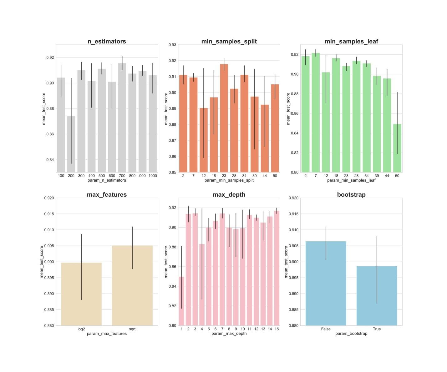
n_estimators: values of 300, 500, 700, apparently, show the best average results.min_samples_split: Small values like 2 and 7 seem to show the best results. The value 23 also looks good. You can examine several values of this hyperparameter in excess of 2, as well as several values of about 23.min_samples_leaf: There is a feeling that small values of this hyperparameter give better results. This means that we can experience values between 2 and 7.max_features: option sqrtgives the highest average result.max_depth: there is no clear relationship between the value of the hyperparameter and the result of the model, but there is a feeling that the values 2, 3, 7, 11, 15 look good.bootstrap: the value Falseshows the best average result.
Now, using these findings, we can move on to the second round of optimization of hyperparameters. This will narrow the range of values we are interested in.8. Optimization of hyperparameters. Round 2: GridSearchCV (final preparation of parameters for model No. 3, RF + PCA + HT)
After applying the RandomizedSearchCV algorithm, we will use the GridSearchCV algorithm to conduct a more accurate search for the best combination of hyperparameters. The same hyperparameters are investigated here, but now we are applying a more “thorough” search for their best combination. Using the GridSearchCV algorithm, each combination of hyperparameters is examined. This requires much more computational resources than using the RandomizedSearchCV algorithm when we independently set the number of search iterations. For example, researching 10 values for each of 6 hyperparameters with cross-validation in 3 blocks will require 10⁶ x 3, or 3,000,000 model training sessions. That is why we use the GridSearchCV algorithm after, after applying RandomizedSearchCV, we narrowed the ranges of the values of the studied parameters.So, using what we found out with the help of RandomizedSearchCV, we examine the values of the hyperparameters that have shown themselves best:from sklearn.model_selection import GridSearchCV
n_estimators = [300,500,700]
max_features = ['sqrt']
max_depth = [2,3,7,11,15]
min_samples_split = [2,3,4,22,23,24]
min_samples_leaf = [2,3,4,5,6,7]
bootstrap = [False]
param_grid = {'n_estimators': n_estimators,
'max_features': max_features,
'max_depth': max_depth,
'min_samples_split': min_samples_split,
'min_samples_leaf': min_samples_leaf,
'bootstrap': bootstrap}
gs = GridSearchCV(rfc_2, param_grid, cv = 3, verbose = 1, n_jobs=-1)
gs.fit(X_train_scaled_pca, y_train)
rfc_3 = gs.best_estimator_
gs.best_params_
Here we apply cross-validation in 3 blocks for 540 (3 x 1 x 5 x 6 x 6 x 1) model training sessions, which gives 1620 model training sessions. And now, after we used RandomizedSearchCV and GridSearchCV, we can turn to the attribute best_params_to find out which values of hyperparameters allow the model to work best with the data set under study (these values can be seen at the bottom of the previous code block) . These parameters are used to create model number 3.9. Evaluation of the quality of the models on the verification data
Now you can evaluate the created models on the verification data. Namely, we are talking about those three models described at the very beginning of the material.Check out these models:y_pred = rfc.predict(X_test_scaled)
y_pred_pca = rfc.predict(X_test_scaled_pca)
y_pred_gs = gs.best_estimator_.predict(X_test_scaled_pca)
Create error matrices for the models and find out how well each of them is able to predict breast cancer:from sklearn.metrics import confusion_matrix
conf_matrix_baseline = pd.DataFrame(confusion_matrix(y_test, y_pred), index = ['actual 0', 'actual 1'], columns = ['predicted 0', 'predicted 1'])
conf_matrix_baseline_pca = pd.DataFrame(confusion_matrix(y_test, y_pred_pca), index = ['actual 0', 'actual 1'], columns = ['predicted 0', 'predicted 1'])
conf_matrix_tuned_pca = pd.DataFrame(confusion_matrix(y_test, y_pred_gs), index = ['actual 0', 'actual 1'], columns = ['predicted 0', 'predicted 1'])
display(conf_matrix_baseline)
display('Baseline Random Forest recall score', recall_score(y_test, y_pred))
display(conf_matrix_baseline_pca)
display('Baseline Random Forest With PCA recall score', recall_score(y_test, y_pred_pca))
display(conf_matrix_tuned_pca)
display('Hyperparameter Tuned Random Forest With PCA Reduced Dimensionality recall score', recall_score(y_test, y_pred_gs))
Results of the work of the three modelsHere the metric “completeness” (recall) is evaluated. The fact is that we are dealing with a diagnosis of cancer. Therefore, we are extremely interested in minimizing false negative forecasts issued by models.Given this, we can conclude that the basic RF model gave the best results. Its completeness rate was 94.97%. In the test dataset, there was a record of 179 patients who have cancer. The model found 170 of them.Summary
This study provides an important observation. Sometimes the RF model, which uses the principal component method and large-scale optimization of hyperparameters, may not work as well as the most ordinary model with standard settings. But this is not a reason to limit yourself to only the simplest models. Without trying different models, it is impossible to say which one will show the best result. And in the case of models that are used to predict the presence of cancer in patients, we can say that the better the model - the more lives can be saved.Dear readers! What tasks do you solve using machine learning methods?