💅🏿 🖖 👈🏾 Visualization of lines of tension and movements of electrostatic charges, simulation of planetary motion of the solar system 🐕 👸🏾 👩🏾‍🤝‍👨🏽

Hi, today I want to offer you a visual aid for modeling some physical processes and show how to get beautiful images and animations. Caution a lot of pictures.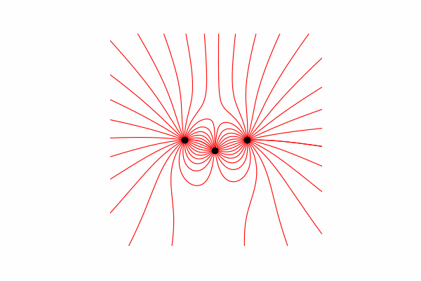

All code can be found in google colab .

Theory

First, we need a small theoretical minimum on this topic. Let's start by understanding what tension lines are and how to count them. In fact, these lines are the merger of many tension vectors, which can be calculated as follows:

E = f r a c k * | q | r^{2}

$E = \ frac {k * | q |} {r ^ 2}$ .

E calculation method

I calculated the tension vector through the similarity of triangles, thereby obtaining projections on the x and y axes dx and dy, respectively.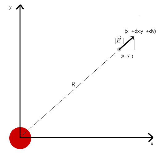

From the similarity it follows that the radius of the vector from the charge to the point in space r and the length of the intensity vector E is equal to the ratio of the projections of these vectors (x1 and dx, respectively)

f r a c R E = f r a c x d x = f r a c y d y

$\ frac {R} {E} = \ frac {x} {dx} = \ frac {y} {dy}$ . Formula of the resulting vector

v e c E = l e f t (b e g i n a r r a y c s u m_{i = 0}^{N} f r a c x_{i} * | v e c E_{i} | R_{i} s u m_{i = 0}^{N} f r a c y_{i} * | v e c E_{i} | R_{i} e n d a r r a y r i g h t) q q u a d

$\ vec {E} = \ left (\ begin {array} {c} \ sum_ {i = 0} ^ {N} \ frac {x_i * | \ vec {E} _i |} {R_i} \\ \ sum_ {i = 0} ^ {N} \ frac {y_i * | \ vec {E} _i |} {R_i} \ end {array} \ right) \ qquad$
with this knowledge we get the first result.

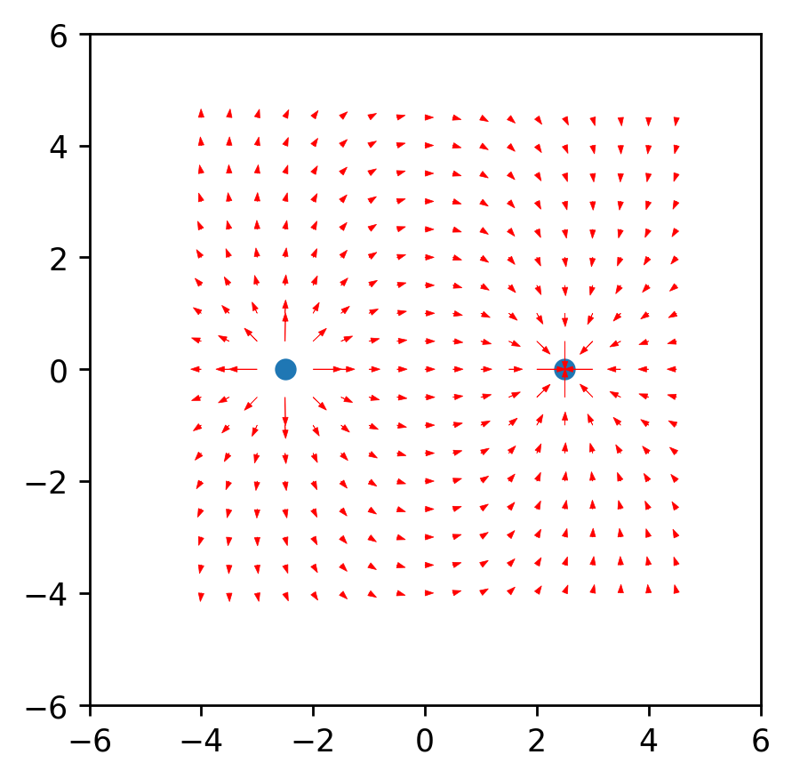
Projection Calculation Function

def E(q_prop, xs, ys, nq): #q_prop=[[xq1, yq1, q1, mq1, vxq1, vyq1], [xq2, yq2, q2, mq2, vxq2, vyq2] ... ] 
    l=1
    k=9*10**9
    Ex=0
    Ey=0
    c=0
    for c in range(len(q_prop)):#                
        q=q_prop[c]
        r=((xs-q[0])**2+(ys-q[1])**2)**0.5
        dEv=(k*q[2])/r**2
        dEx=(xs-q[0])*(dEv/r)*l
        dEy=(ys-q[1])*(dEv/r)*l

        Ex+=dEx
        Ey+=dEy
    return Ex, Ey

Line construction method

First you need to decide on the start and end point where the line and the doc will go from. The beginning is points on a circle with a radius r around the charge, and the end points are no more than r apart from the charges.

code for starting points

theta = np.linspace(0, 2*np.pi, n)
mask=q_prop[ q_prop[:,2]>0 ]#    
for cq in range(len(mask)):
    qmask=mask[cq]
    xr = r_q*np.cos(theta)+qmask[0]# -    
    yr = r_q*np.sin(theta)+qmask[1]#

So it’s worth saying that the lines are built only from positive charges.

And finally, the construction of lines. To do this, we build the line of the vector of tension in it from the starting point, update the starting point at the end of the constructed line and repeat until the end conditions mentioned above are reached.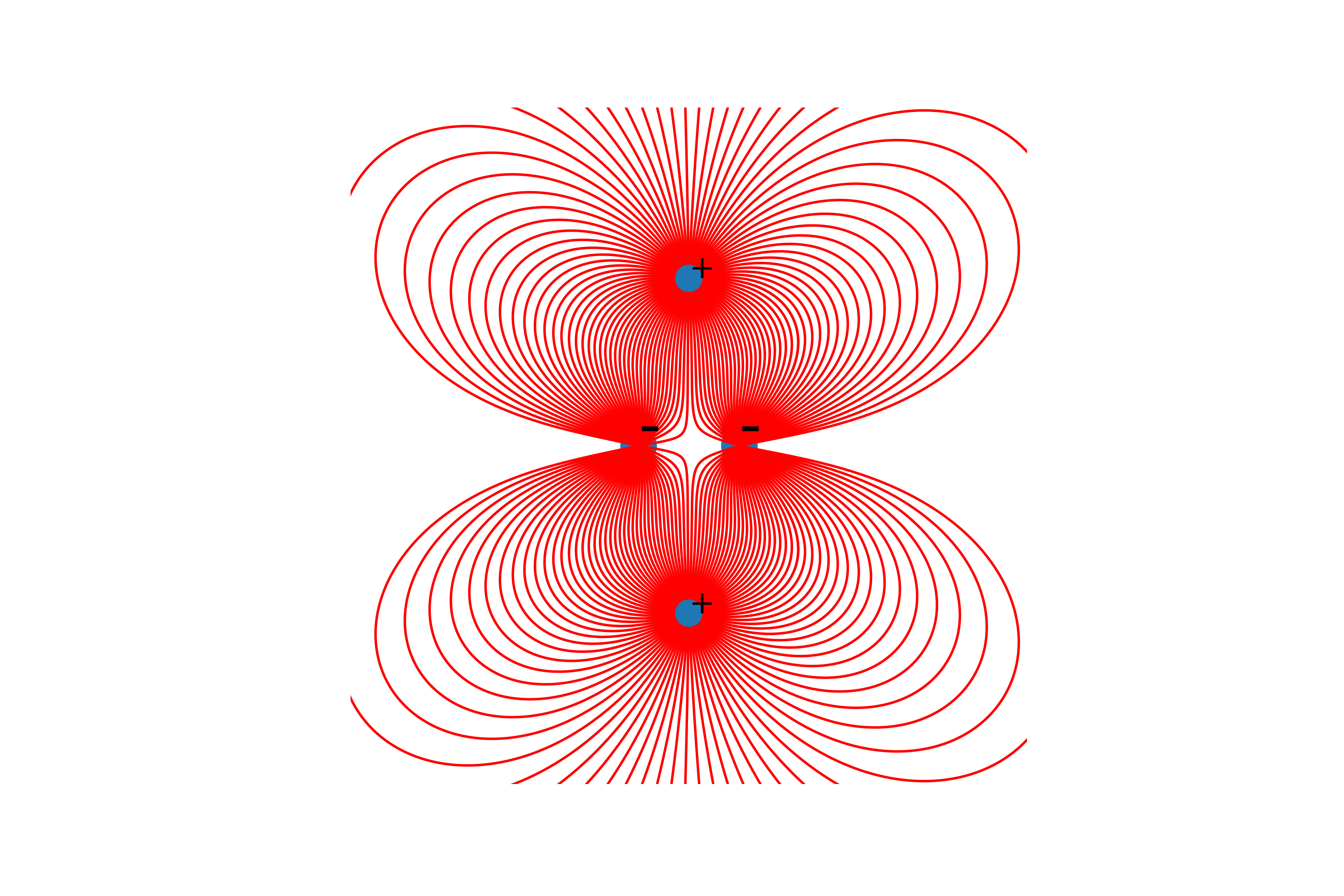

line coordinate calculation function

def Draw(size, q_prop,r_q, n):
  
  linen=np.empty((np.count_nonzero(q_prop[:,2]>0),n, 2000000), dtype=np.float64)
  linen[:] = np.nan
  theta = np.linspace(0, 2*np.pi, n)
  mask=q_prop[ q_prop[:,2]>0 ][ q_prop[q_prop[:,2]>0][:,3]==1 ]
  for cq in range(len(mask)):
    qmask=mask[cq]
    x11 = r_q*np.cos(theta)+qmask[0]
    x22 = r_q*np.sin(theta)+qmask[1]
    for c in range(len(x11)):

      xs=x11[c]
      ys=x22[c]

      lines=np.empty((2,1000000), dtype=np.float64)
      lines[:]=np.nan
      stop=0
      nnn=0
      
      lines[0][nnn]=xs
      lines[1][nnn]=ys
      while  abs(xs)<size+2 and abs(ys)<size+2: 
        nnn+=1

        for cq1 in range(len(q_prop)):
          q=q_prop[cq1]
          if ((ys-q[1])**2+(xs-q[0])**2)**0.5<r_q/2 :
            stop=1
            break
        if stop==1:
          break
        dx, dy = E1(q_prop,xs,ys)

        xs+=dx
        ys+=dy
        lines[0][nnn]=xs
        lines[1][nnn]=ys
       
      linen[cq,c,:]=lines.reshape(-1)

  return linen

Interaction between charges

To reflect their interaction, it is necessary to change its coordinates and speed after each small time dt.

x + = f r a c E_{x} c d o t q c d o t d t^{2} 2 c d o t m + v_{x} c d o t d t

$x + = \ frac {E_x \ cdot q \ cdot dt ^ 2} {2 \ cdot m} + v_x \ cdot dt$

y + = f r a c E_{y} c d o t q c d o t d t^{2} 2 c d o t m + v_{y} c d o t d t

$y + = \ frac {E_y \ cdot q \ cdot dt ^ 2} {2 \ cdot m} + v_y \ cdot dt$

v_{x} + = f r a c E_{x} c d o t q c d o t d t m

$v_x + = \ frac {E_x \ cdot q \ cdot dt} {m}$

v_{y} + = f r a c E_{y} c d o t q c d o t d t m

$v_y + = \ frac {E_y \ cdot q \ cdot dt} {m}$

Function for updating coordinates and projections of charge speeds

def Update_all(q_prop):
  vx=0
  vy=0
  x=0
  y=0
  q_prop_1=np.copy(q_prop)
  for c in range(len(q_prop)):#         
    xs=q_prop[c][0]
    ys=q_prop[c][1]
    q =q_prop[c][2]
    m =q_prop[c][3]
    vx=q_prop[c][4]
    vy=q_prop[c][5]
    Ex, Ey= E(q_prop, xs, ys, c)

    x=(((Ex*q)/m)*dt**2)/2+vx*dt+xs
    y=(((Ey*q)/m)*dt**2)/2+vy*dt+ys
    vx+=((Ex*q)/m)*dt
    vy+=((Ey*q)/m)*dt
    #print(q_prop[c]-[x,y,q,m,vx,vy])
    q_prop_1[c]=[x,y,q,m,vx,vy]
  
  return q_prop_1#

Gravity

Based on the existing code, I wrote a simulator that reflects the movements of bodies under the influence of gravity. Changes in the code are mainly for the tension function since acceleration will now be considered using a similar formula.

g = f r a c G * m r^{2}

$g = \ frac {G * m} {r ^ 2}$

v e c g = l e f t (b e g i n a r r a y c s u m_{i = 0}^{N} f r a c x_{i} * | v e c g_{i} | R_{i} s u m_{i = 0}^{N} f r a c y_{i} * | v e c g_{i} | R_{i} e n d a r r a y r i g h t) q q u a d

$\ vec {g} = \ left (\ begin {array} {c} \ sum_ {i = 0} ^ {N} \ frac {x_i * | \ vec {g} _i |} {R_i} \\ \ sum_ {i = 0} ^ {N} \ frac {y_i * | \ vec {g} _i |} {R_i} \ end {array} \ right) \ qquad$

Planets start from the x axis at perihelion distance and at perihelion speed. All the values of the planets and the sun (mass, distance, extremities) from the directory.

Animation for the first 4 planets + sun.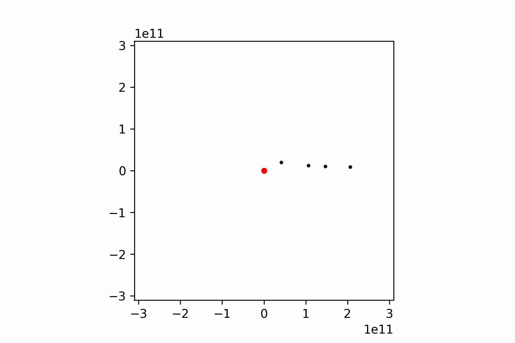

Waiting for criticism and suggestions. Bye.

Visualization of lines of tension and movements of electrostatic charges, simulation of planetary motion of the solar system

Theory

E calculation method

Line construction method

Interaction between charges

Gravity

More articles: