👍🏻 🚚 ™️ Understanding the machine learning model that breaks CAPTCHA 🤳 🤵🏿 👩🏻‍🎨

Hello everyone! This month, OTUS is recruiting a new group on the Machine Learning course . According to established tradition, on the eve of the start of the course, we are sharing with you the translation of interesting material on the topic.

Computer vision is one of the most relevant and researched topics of AI [1], however, current methods for solving problems using convolutional neural networks are seriously criticized due to the fact that such networks are easily fooled. In order not to be unfounded, I’ll tell you about several reasons: networks of this type give an incorrect result with high confidence for naturally occurring images that do not contain statistical signals [2], which convolutional neural networks rely on, for images that were previously correctly classified, but in which one pixel [3] or images with physical objects that were added to the scene but did not have to change the classification result [4] changed. The fact is, if we want to create truly intelligent machines,it should seem reasonable to us to invest in the study of new ideas.

One of these new ideas is Vicarious’s application of the Recursive Cortical Network (RCN), which draws inspiration from neuroscience. This model claimed to be extremely effective at breaking text captcha, thereby causing a lot of talk around itself . Therefore, I decided to write several articles, each of which explains a certain aspect of this model. In this article, we will talk about its structure and how the generation of images presented in the materials of the main article on RCN [5] is generated.

This article assumes that you are already familiar with convolutional neural networks, so I will draw many analogies with them.

To prepare for RCN awareness, you need to understand that RCNs are based on the idea of separating the shape (sketch of the object) from the appearance (its texture) and that it is a generative model, not a discriminant one, so we can generate images using it, as in a generative adversarial networks. In addition, a parallel hierarchical structure is used, similar to the architecture of convolutional neural networks, which begins with the stage of determining the shape of the target object in the lower layers, and then its appearance is added to the upper layer. Unlike convolutional neural networks, the model we are considering relies on a rich theoretical base of graphical models, instead of weighted sums and gradient descent. Now let's delve into the features of the RCN structure.

Feature layers

The first type of layer in RCN is called the feature layer. We will consider the model gradually, so let's assume for now that the entire hierarchy of the model consists only of layers of this type stacked on top of each other. We will move from high-level abstract concepts to more specific features of the lower layers, as shown in Figure 1 . A layer of this type consists of several nodes located in two-dimensional space, similarly to feature maps in convolutional neural networks.

Figure 1 : Several feature layers located one above the other with nodes in two-dimensional space. The transition from the fourth to the first layer means the transition from the general to the particular.

Each node consists of several channels, each of which represents a separate feature. Channels are binary variables that take the value True or False, indicating whether an object corresponding to this channel exists in the final generated image in the coordinate (x, y) of the node. At any level, nodes have the same type of channels.

As an example, let's take an intermediate layer and talk about its channels and the layers above to simplify the explanation. The list of channels on this layer will be a hyperbola, a circle and a parabola. On a certain run when generating the image, the calculations of the overlying layers required a circle in the coordinate (1,1). Thus, the node (1, 1) will have a channel corresponding to the object “circle” in the value True. This will directly affect some nodes in the layer below, that is, the lower level features that are associated with the circle in the neighborhood (1,1) will be set to True. These lower level objects can be, for example, four arcs with different orientations. When the features of the lower layer are activated, they activate the channels on the layers even lower until the last layer is reached,image generating. Activation visualization is shown inFigure 2 .

You may ask, how will it become clear that the representation of a circle is 4 arcs? And how does RCN know that it needs a channel to represent the circle? Channels and their bindings to other layers will be formed at the RCN training stage.

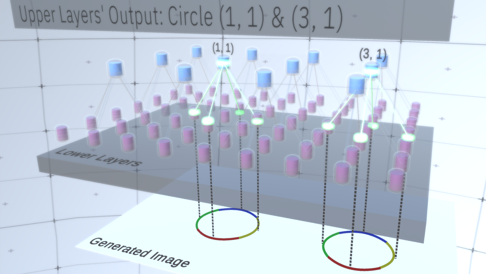Figure 2: Information flow in feature layers. Nodes of signs are capsules containing disks representing channels. Some of the upper and lower layers were presented in the form of a parallelepiped for simplicity, however, in reality they also consist of feature nodes as intermediate layers. Please note that the upper intermediate layer consists of 3 channels, and the second layer consists of 4 channels.

You may indicate a very rigid and deterministic method for generating the adopted model, but for people, small perturbations of the curvature of the circle are still considered to be a circle, as you can see in Figure 3 .

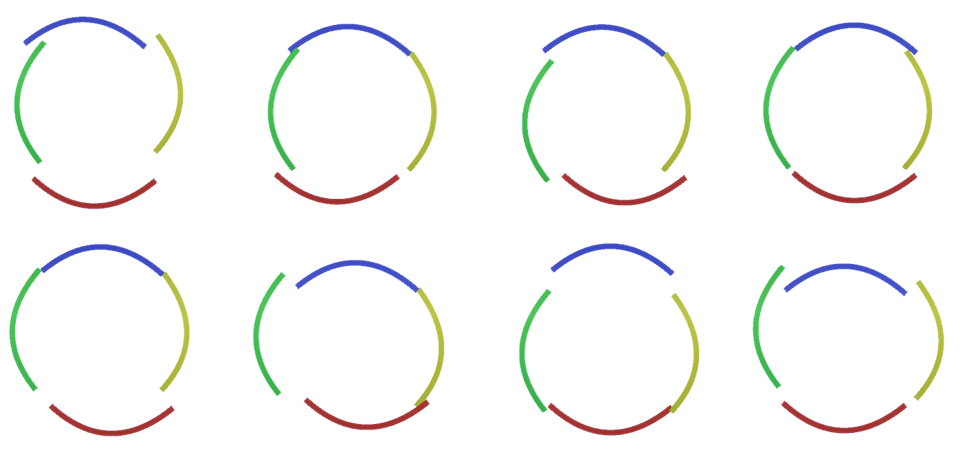Figure 3: Many variations of the construction of a circle of four curved arcs from Figure 2.

It would be difficult to consider each of these variations as a separate new channel in the layer. Similarly, grouping variations into the same entity will greatly facilitate generalization into new variations when we adapt RCN to classification instead of generation a little later. But how do we change RCN to get this opportunity?

Subsampling layers

To do this, you need a new type of layer - the pooling layer. It is located between any two layers of signs and acts as an intermediary between them. It also consists of channels, however they have integer values, not binary ones.

To illustrate how these layers work, let's go back to the circle example. Instead of requiring 4 arcs with fixed coordinates from the feature layer above it as a feature of a circle, the search will be performed on the subsample layer. Then, each activated channel in the subsample layer will select a node on the underlying layer in its vicinity to allow for slight distortion of the feature. Thus, if we establish communication with 9 nodes directly below the subsample node, the subsample channel, whenever it is activated, will evenly select one of these 9 nodes and activate it, and the index of the selected node will be the state of the subsample channel - an integer. In Figure 4you can see several runs, where each run uses a different set of lower-level nodes, respectively, allowing you to create a circle in various ways.

Figure 4: Operation of subsampling layers. Each frame in this GIF picture is a separate launch. Subsampling nodes are cubed. In this image, the subsample nodes have 4 channels equivalent to 4 channels of the feature layer below it. The upper and lower layers were completely removed from the picture.

Despite the fact that we needed the variability of our model, it would be better if it remained more restrained and focused. In the previous two figures, some circles look too strange to really interpret them as circles due to the fact that the arcs are not interconnected, as can be seen from Figure 5. We would like to avoid generating them. Thus, if we could add a mechanism for subsampling channels to coordinate the selection of feature nodes and focus on continuous forms, our model would be more accurate.

Figure 5: Many options for constructing a circle. Those options that we want to drop are marked with red crosses.

RCN authors used lateral connection in subsampling layers for this purpose. Essentially, subsampling channels will have links with other subsampling channels from the immediate environment, and these links will not allow some pairs of states to coexist in two channels simultaneously. In fact, the sample area of these two channels will simply be limited. In various versions of the circle, these connections, for example, will not allow two adjacent arcs to move away from each other. This mechanism is shown in Figure 6.. Again, these relationships are established at the training stage. It should be noted that modern vanilla artificial neural networks do not have any lateral connections in their layers, although they do exist in biological neural networks and it is assumed that they play a role in the contour integration in the visual cortex (but, frankly, the visual cortex has more complex device than it might seem from the previous statement).

Figure 6: GIF- RCN . , . , RCN , , . .

So far, we talked about intermediate layers of RCN, we have only the topmost layer and the lowest layer that interacts with the pixels of the generated image. The topmost layer is a regular feature layer, where the channels of each node will be classes of our labeled dataset. When generating, we simply select the location and the class that we want to create, go to the node with the specified location and say that it activates the channel of the class we selected. This activates some of the channels in the subsample layer below it, then the feature layer below, and so on, until we reach the last feature layer. Based on your knowledge of convolutional neural networks, you should think that the topmost layer will have a single node, but this is not so, and this is one of the advantages of RCN,but a discussion of this topic is beyond the scope of this article.

The last feature layer will be unique. Remember, I talked about how RCNs separate form from appearance? It is this layer that will be responsible for obtaining the shape of the generated object. Thus, this layer should work with very low-level features, the most basic building blocks of any shape, which will help us generate any desired shape. Small borders rotating at different angles are quite suitable, and it is precisely them that the authors of the technology use.

The authors selected the attributes of the last level to represent a 3x3 window that has a border with a certain rotation angle, which they call a patch descriptor. The number of rotation angles that they chose is 16. In addition, in order to be able to add an appearance later, you need two orientations for each rotation in order to be able to tell whether the background is on the left or on the right border, if these are external borders , and additional orientation in the case of internal boundaries (i.e., inside the object). In Figure 7 shows the characteristics of the last layer assembly, and Figure 8 shows how the descriptors of patches can generate certain shape.

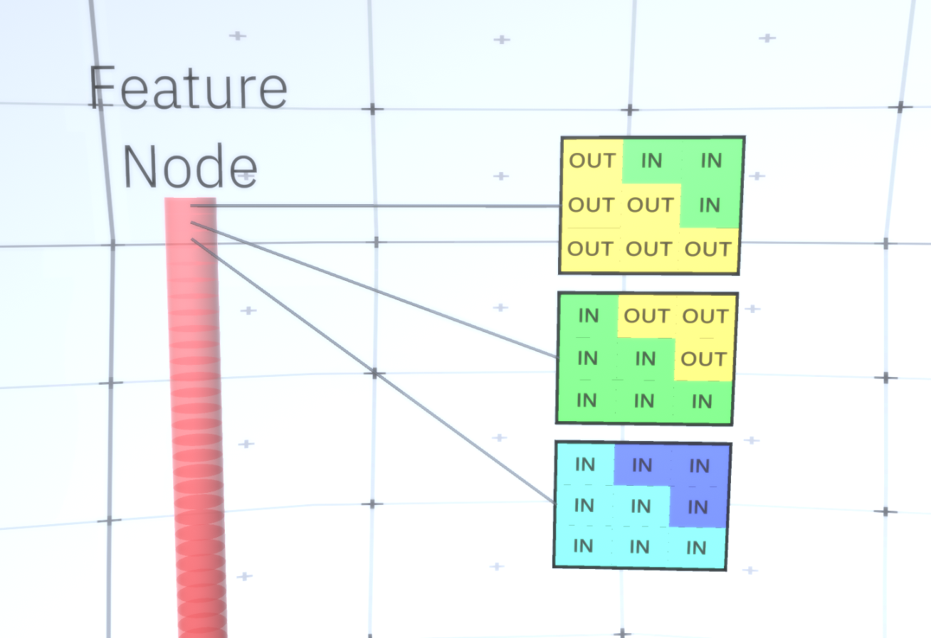Figure 7: . 48 ( ) , 16 3 . – 45 . “IN " , “OUT” — .

8: «i» .

Now that we have reached the last layer of signs, we have a diagram on which the boundaries of the object are determined and the understanding of whether the area is outside the border is internal or external. It remains to add an appearance, designating each remaining area in the image as IN or OUT and paint over the area. A conditional random field may help here. Without going into mathematical details, we simply assign to each pixel in the final image a probability distribution by color and state (IN or OUT). This distribution will reflect information obtained from the border of the map. For example, if there are two adjacent pixels, one of which is IN, and the other is OUT, the likelihood that they will have a different color increases greatly. If two adjacent pixels are on opposite sides of the inner border, the probabilitythat will have a different color will also increase. If the pixels lie inside the border and are not separated by anything, then the likelihood that they have the same color increases, but the external pixels may have a slight deviation from each other and so on. To get the final image, you just make a selection from the joint probability distribution that we just installed. To make the generated image more interesting, we can replace the colors with the texture. We will not discuss this layer because RCN can perform the classification without being based on appearance.To get the final image, you just make a selection from the joint probability distribution that we just installed. To make the generated image more interesting, we can replace the colors with the texture. We will not discuss this layer because RCN can perform the classification without being based on appearance.To get the final image, you just make a selection from the joint probability distribution that we just installed. To make the generated image more interesting, we can replace the colors with the texture. We will not discuss this layer because RCN can perform the classification without being based on appearance.

Well, we will end here for today. If you want to know more about RCN, read this article [5] and the appendix with additional materials, or you can read my other articles on the logical conclusions , training and results of using RCN on various datasets .

Sources:

: « : ».

Understanding the machine learning model that breaks CAPTCHA

Feature layers

Subsampling layers

Sources:

More articles: