R is a very powerful tool for working with statistics: from pre-processing to building models of any complexity and corresponding graphics.
A simple Google request will provide a large amount of literature on how to “use R easily and quickly.” There will be huge books and numerous notes on the Stack Overflow , which, at first glance, seem like an endless storehouse of examples, each of which in two counts will collect the necessary code to solve a specific problem. However, in reality this is not at all true. There are very few materials that would tell, for example, how to build a simple schedule “from scratch” with ready-made recipes for solving difficulties that will arise in the course of solving this problem.
To solve practical problems, specific step-by-step instructions are needed, and not a detailed description of the full power of a package. In addition, ready-made training examples (the same irises ) are often of little use, since they immediately skip one of the most important stages of working with statistics - the preliminary collection and processing of the data itself. But it is precisely for this work that almost a large part of all time often takes! A separate problem is the creation of schedules that correspond to formal, and more often informal, standards of a certain professional environment.
My colleagues and I regularly need to do more and more visualizations of statistics and models based on them to publish scientific results. Since the studies concern economics, many of these works are similar to professional journalism.
At some point, it became clear that for effective teamwork a kind of full-fledged statistics processing pipeline is needed. This article was born as an introductory guide for colleagues and a cheat sheet for myself to run this conveyor. It seems that this material can be useful to a wider audience.
R Pain-Free Graphics: Walkthrough
Basic setting R
: R + RStudio. . R, RStudio. .
- R , ( Session — Set Working Directory — To Source File Location). , RStudio . - RStudio , .
R ( plot), , , .
R ggplot2, .
readxl ( .xls, .xlsx) dplyr ( ), scales ( ), Cairo ( ggplot ). :
install.packages("ggplot2", "readxl", "scales", "dplyr", "Cairo")
, , , . , , , .
:
- ?
- ?
: CSV Microsoft Excel ( , «» .xlsx » .xls). , CSV ( , , ) . Excel : -, , -, , . CSV R , .
— , , . , , . , R . , , , . , , : year (), var ( ), value ( ).
.
: , 2009—2018 .
: - . . .xlsx , . , (, ) , , .
, «» ( ) , «» «» «». , . Excel ( ) , , , ( , R , ). ( ).
logging, graphs.xlsx RStudio.
.
library(ggplot2)
library(readxl)
library(Cairo)
library(scales)
library(dplyr)
, . , — , , UTF-8:
Sys.setlocale("LC_ALL", "ru_RU.UTF-8")
(- Windows Linux), , — , .
R.
df_logging <- read_excel("graphs.xlsx", sheet ="logging")
sheet Excel, .
.
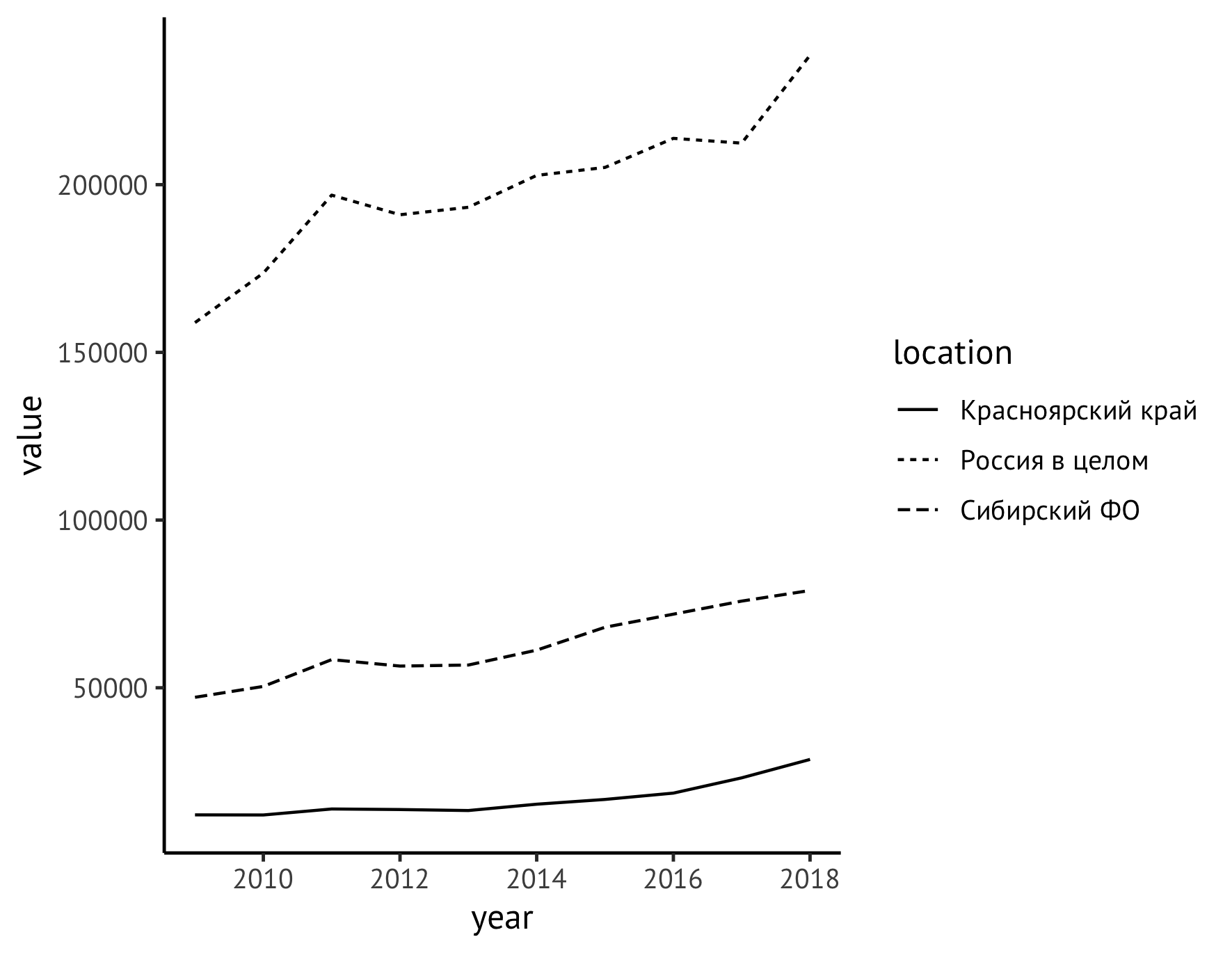
ggplot(data=df_logging, aes(x=year, y=value)) +
    geom_line(aes(linetype=location))

, « » , , .
. ggplot2 . theme_classic. . PT Sans, PT Serif, PT Mono. , , Times Helvetica. , , , . 12 .
ggplot(data=df_logging, aes(x=year, y=value)) +
    geom_line(aes(linetype=location)) +
    theme_classic(base_family = "PT Sans", base_size = 12)
( theme) ( labs). Y (« , . »), X , , .
ggplot(data=df_logging, aes(x=year, y=value)) +
    geom_line(aes(linetype=location)) +
    theme_classic(base_family = "PT Sans", base_size = 12) +
    theme(legend.title = element_blank(), legend.position="bottom", legend.spacing.x = unit(0.5, "lines")) +
    labs(x = "", y = " , . . ", color="")

, . . . 1000, :
ggplot(data=df_logging, aes(x=year, y=value/1000))
:
labs(x = "", y = " , . ", color="")
, , :
geom_point(size=2)
. , — :
scale_linetype_manual(values=c("twodash", "solid", "dotted"))
:
ggplot(data=df_logging, aes(x=year, y=value/1000)) +
    geom_line(aes(linetype=location)) +
    geom_point(size=1) +
    theme_classic(base_family = "PT Sans", base_size = 12) +
    theme(legend.title = element_blank(), legend.position="bottom", legend.spacing.x = unit(0.5, "lines")) +
    scale_linetype_manual(values=c("twodash", "solid", "dotted")) +
    labs(x = "", y = " ,  . ", color="")

— . , , 2014 , . , , , 2011-. geom_text:
geom_text(aes(label=format(value/1000, digits = 3, decimal.mark = ",")),
    data = subset(df_logging, year == 2009 | year == 2018 | year == 2011),
    check_overlap = TRUE, vjust=-0.8)
, , , . , . geom_text . data. df_logging, . , , , , . , : 2009 ( ), 2011 ( ), 2018 ( ). subset.
(decimal.mark), — digits. , round , , digits 3.
check_overlap , : . vjust . , .
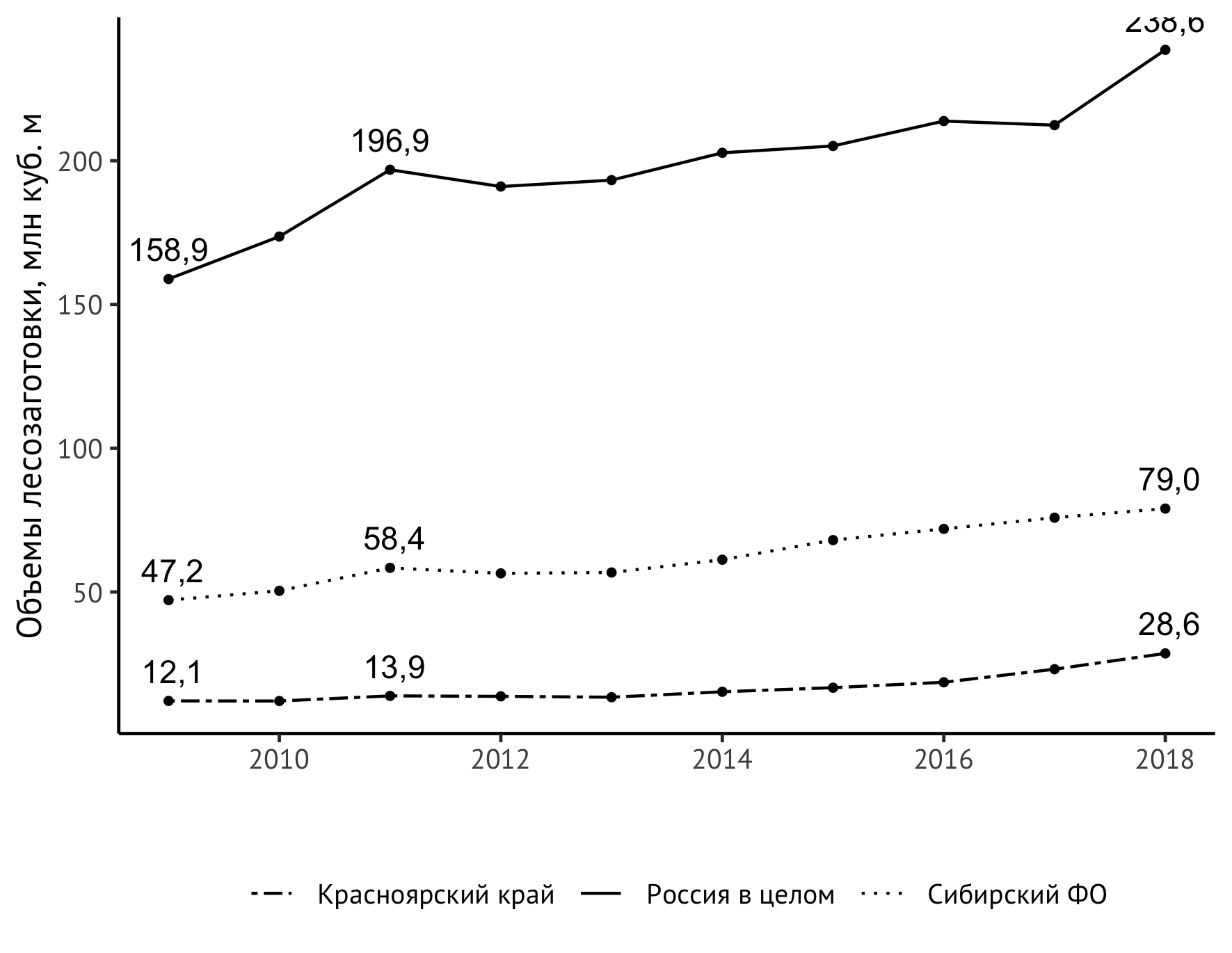
!
— «» . . 250 . :
scale_y_continuous(limits = c(0,250))
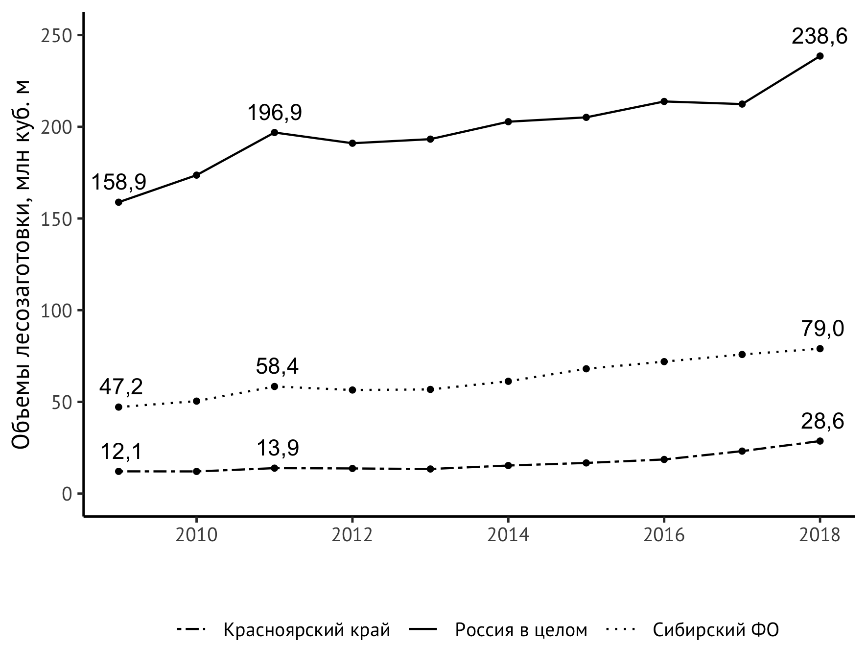
! , :
ggplot(data=df_logging, aes(x=year, y=value/1000)) +
    geom_line(aes(linetype=location)) +
    geom_point(size=1) +
    theme_classic(base_family = "PT Sans", base_size = 12) +
    theme(legend.title = element_blank(), legend.position="bottom", legend.spacing.x = unit(0.5, "lines")) +
    geom_text(aes(label=format(value/1000, digits = 3, decimal.mark = ",")),
data = subset(df_logging, year == 2009 | year == 2018 | year == 2011),
check_overlap = TRUE, vjust=-0.8) +
    geom_text(aes(label=format(value/1000, digits = 3, decimal.mark = ",")),
    data = subset(df_logging, year == 2009 | year == 2018 | year == 2011),
    check_overlap = TRUE, vjust=-0.8) +
    scale_linetype_manual(values=c("twodash", "solid", "dotted")) +
    scale_y_continuous(limits = c(0,250)) +
    labs(x = "", y = " ,  . ", color="")
: ( ) / . . . — : , 2020 ( ).
RStudio , . , . (.jpg, .png), , , , Word, . .eps .pdf : , , .
ggsave ggplot.
, , .png, :
ggsave("logging.png", width=709, height=549, units="px")
( width height) (units) , , . , .
, . .eps — Word. Cairo:
ggsave(filename = "export.eps", width=15, height=11.6, units="cm", device = cairo_ps)
, R.
R . , ggplot:
, R . R. , R.
You can also recommend a book in Russian about R in general:
Shitikov V.K., Mastitsky S.E. Classification, regression, Data Mining algorithms using R. 2017 .
Just an interesting and motivating example is a powerful presentation on the use of ggplot2 in preparing drawings for the influential newspaper Financial Times .