Analyse der Popularität von YouTube-Videos von Eurovision 2020-Teilnehmern

Am 13. März wurde auf dem offiziellen Eurovision-YouTube-Kanal die Zusammensetzung der Little Big-Gruppe veröffentlicht, die Russland beim Wettbewerb vertreten wird. Nachdem ich mir den Clip angesehen hatte, wollte ich die Statistiken des Videos unserer Gruppe mit den Videos anderer Teilnehmer vergleichen. Welche Videos werden am häufigsten angesehen, wer hat den höchsten Prozentsatz an Likes, wer wird am häufigsten kommentiert? Das Googeln der fertigen Statistiken führte zu nichts. Daher wurde beschlossen, die erforderlichen Statistiken zu sammeln.

Artikelstruktur:

• Code hochladen
• Analyse
• Update am 14.03.2020 20:30
• Zusätzlich: Wir untersuchen die Abhängigkeit der Ansichten von der Bevölkerung des Landes

Wenn Sie die Wiedergabeliste der Teilnehmer öffnen, sehen Sie 39 Videos. Tatsächlich gibt es 38 Songs. Die Komposition Hurricane - Hasta La Vista - Serbien wurde zweimal heruntergeladen, sodass die Statistiken dazu zusammengefasst werden. Um Statistiken zu sammeln, verwenden wir R.

Code hochladen

Wir benötigen folgende Pakete:

library(tuber) #    API YouTube,     
library(dplyr) #     
library(ggplot2) #  

Gehen Sie zunächst zur Google-Entwicklerkonsole und erstellen Sie einen OAuth-Schlüssel in der YouTube Data API v3-API. Nachdem Sie den Schlüssel erhalten haben, melden Sie sich bei R an.

yt_oauth(" ", "  ")

Jetzt können wir Statistiken sammeln:

#     
list_videos <- get_playlist_items(filter = c(playlist_id = "PLmWYEDTNOGUL69D2wj9m2onBKV2s3uT5Y"))

#    ,  get_stats
stats_videos <- lapply(as.character(list_videos$contentDetails.videoId), get_stats) %>% 
  bind_rows()
stats_videos <- stats_videos %>% 
  mutate_at(vars(-id), as.integer)

#   ,  get_video_details
description_videos <- lapply(as.character(list_videos$contentDetails.videoId), get_video_details)
description_videos <- lapply(description_videos, function(x) {
    list(
      id = x[["items"]][[1]][["id"]],
      name_video = x[["items"]][[1]][["snippet"]][["title"]]
    )
  }) %>% 
  bind_rows()

.. — — [ ] — Official Music Video — Eurovision 2020, , . .

#     
description_videos$name_video <- description_videos$name_video %>% 
  gsub("[^[:alnum:][:blank:]?&/\\-]", '', .) %>% 
  gsub("(  .*)|( - Offic.*)", '', .)

#      
df <- description_videos %>% 
  left_join(stats_videos, by = 'id') %>% 
  rowwise() %>% 
  mutate( #   
    proc_like = round(likeCount / (likeCount + dislikeCount), 2)
    ) %>% 
  ungroup()

# Hurricane - Hasta La Vista - Serbia     ,  
df <- df %>% 
  group_by(name_video) %>% 
  summarise(
    id = first(id),
    viewCount = sum(viewCount),
    likeCount = sum(likeCount),
    dislikeCount = sum(dislikeCount),
    commentCount = sum(commentCount),
    proc_like = round(likeCount / (likeCount + dislikeCount), 2)
  )

df$color <- ifelse(df$name_video == 'Little Big - Uno - Russia','red','gray')

. .

# - 
ggplot(df, aes(x = reorder(name_video, viewCount), y = viewCount, fill = color)) +
  geom_col() +
  coord_flip() +
  theme_light() +
  labs(x = NULL, y = "- ") +
  guides(fill = F) +
  scale_fill_manual(values = c('gray', 'red')) +
  scale_y_continuous(labels = scales::number_format(big.mark = " "))

#    
ggplot(df, aes(x = reorder(name_video, proc_like), y = proc_like, fill = color)) +
  geom_col() +
  coord_flip() +
  theme_light() +
  labs(x = NULL, y = "   ") +
  guides(fill = F) +
  scale_fill_manual(values = c('gray', 'red')) +
  scale_y_continuous(labels = scales::percent_format(accuracy = 1))

# - 
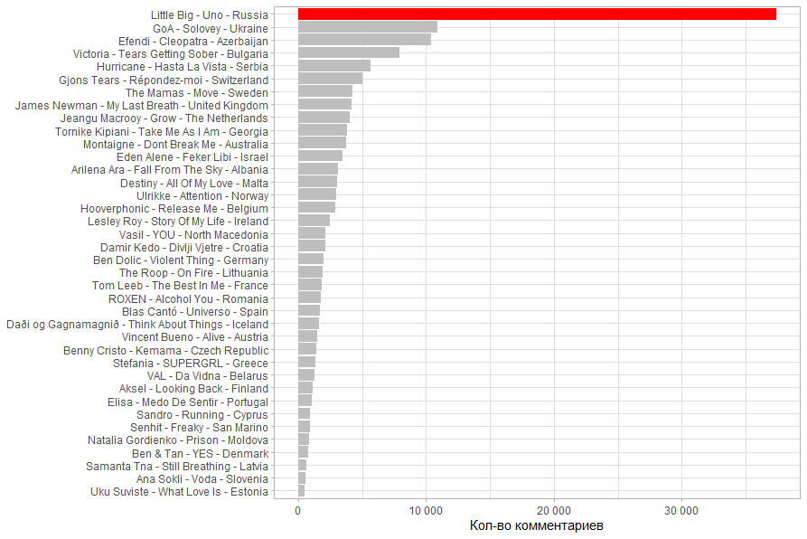
ggplot(df, aes(x = reorder(name_video, commentCount), y = commentCount, fill = color)) +
  geom_col() +
  coord_flip() +
  theme_light() +
  labs(x = NULL, y = "- ") +
  guides(fill = F) +
  scale_fill_manual(values = c('gray', 'red')) +
  scale_y_continuous(labels = scales::number_format(big.mark = " "))

#    
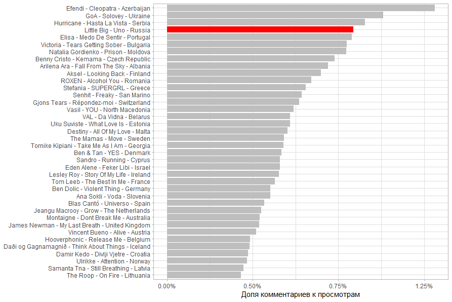
ggplot(df, aes(x = reorder(name_video, commentCount/viewCount), y = commentCount/viewCount, fill = color)) +
  geom_col() +
  coord_flip() +
  theme_light() +
  labs(x = NULL, y = "   ") +
  guides(fill = F) +
  scale_fill_manual(values = c('gray', 'red')) +
  scale_y_continuous(labels = scales::percent_format(accuracy = 0.25))

, Little Big 1 , .

. Little Big , . - .

, . . .

.

( / ). . .

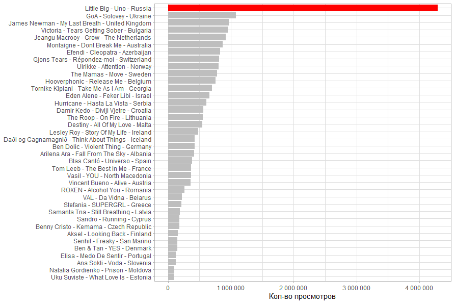
13.03.2020 18:00 , , , .

UPD: 14.03.2020 20:30

. . Little Big , .

, . Little Big ,

.

( / ). 2 , , , . .

14.03.2020 20:30 , , , , . .

:

helg1978 . .

library(rvest)
library(tidyr)

#   
hdoc <- read_html('https://en.wikipedia.org/wiki/List_of_countries_and_dependencies_by_population')

tnode <- html_node(hdoc, xpath = '/html/body/div[3]/div[3]/div[4]/div/table')
df_population <- html_table(tnode)

df_population <- df_population %>% filter(`Country (or dependent territory)` != 'World')

df_population$Population <- as.integer(gsub(',','',df_population$Population,fixed = T))

df_population$`Country (or dependent territory)` <- gsub('\\[.*\\]','', df_population$`Country (or dependent territory)`)

df_population <- df_population %>% 
  select(
    `Country (or dependent territory)`,
    Population
    ) %>% 
  rename(Country = `Country (or dependent territory)`)

#       
df2 <- df %>% 
  separate(name_video, c('compozitor', 'name_track', 'Country'), ' - ', remove = F) %>% 
  mutate(Country = ifelse(Country == 'The Netherlands', 'Netherlands', Country)) %>% 
  left_join(df_population, by = 'Country')

#     
cor(df2$viewCount,df2$Population)
ggplot(df2, aes(x = Population, y =  viewCount)) +
  geom_point() +
  theme_light() +
  geom_smooth(method = 'lm') +
  labs(x = ", ", y = "- ") +
  scale_y_continuous(labels = scales::number_format(big.mark = " ")) +
  scale_x_continuous(labels = scales::number_format(big.mark = " "))

#     ,  
cor(df2[df2$Country != 'Russia',]$viewCount,df2[df2$Country != 'Russia',]$Population)
ggplot(df2 %>% filter(Country != 'Russia') , aes(x = Population, y = viewCount)) +
  geom_point() +
  theme_light() +
  geom_smooth(method = 'lm') +
  labs(x = ", ", y = "- ") +
  scale_y_continuous(labels = scales::number_format(big.mark = " ")) +
  scale_x_continuous(labels = scales::number_format(big.mark = " "))

#     , 
cor(df2$viewCount,df2$Population, method = "spearman")
ggplot(df2 , aes(x = rank(Population), y = rank(viewCount))) +
  geom_point() +
  theme_light() +
  geom_smooth(method = 'lm') +
  labs(x = ",  (  1  40)", y = "-  (  1  40)") +
  guides(fill = F)

#     
ggplot(df2, aes(x = reorder(name_video, viewCount/Population), y = viewCount/Population, fill = color)) +
  geom_col() +
  coord_flip() +
  theme_light() +
  labs(x = NULL, y = "    ") +
  guides(fill = F) +
  scale_fill_manual(values = c('gray', 'red')) +
  scale_y_continuous(labels = scales::percent_format(accuracy = 0.25))

, , 50 . 71%.

. 71% 15%. .

( ), , (. . 40%).

Und als Referenz habe ich den Anteil der Ansichten der Bevölkerung des Landes berechnet. Für besonders kleine Länder stellt sich heraus, dass sie mehr aus anderen Ländern beobachtet wurden. Insbesondere sind es Malta, San Marino und Island.

Voller Github-Code