Quelle: https://mlr3book.mlr-org.com/
Hallo Habr!In diesem Beitrag werden wir den durchdachtesten Ansatz für maschinelles Lernen in der heutigen R-Sprache betrachten - das mlr3- Paket und das Ökosystem um es herum. Dieser Ansatz basiert auf „normalem“ OOP unter Verwendung von R6-Klassen und auf der Darstellung aller Operationen mit Daten und Modellen in Form eines Berechnungsdiagramms. Auf diese Weise können Sie optimierte und flexible Pipelines für maschinelle Lernaufgaben erstellen. Dies kann jedoch zunächst kompliziert und verwirrend erscheinen. Im Folgenden werden wir versuchen, Klarheit zu schaffen und zu motivieren, mlr3 in Ihren Projekten zu verwenden.Inhalt:
- Ein bisschen Geschichte und Vergleich mit konkurrierenden Lösungen
- Technische Details: R6-Klassen und data.table-Paket
- Die Hauptkomponenten der ML-Pipline in mlr3
- Hyperparameter einstellen
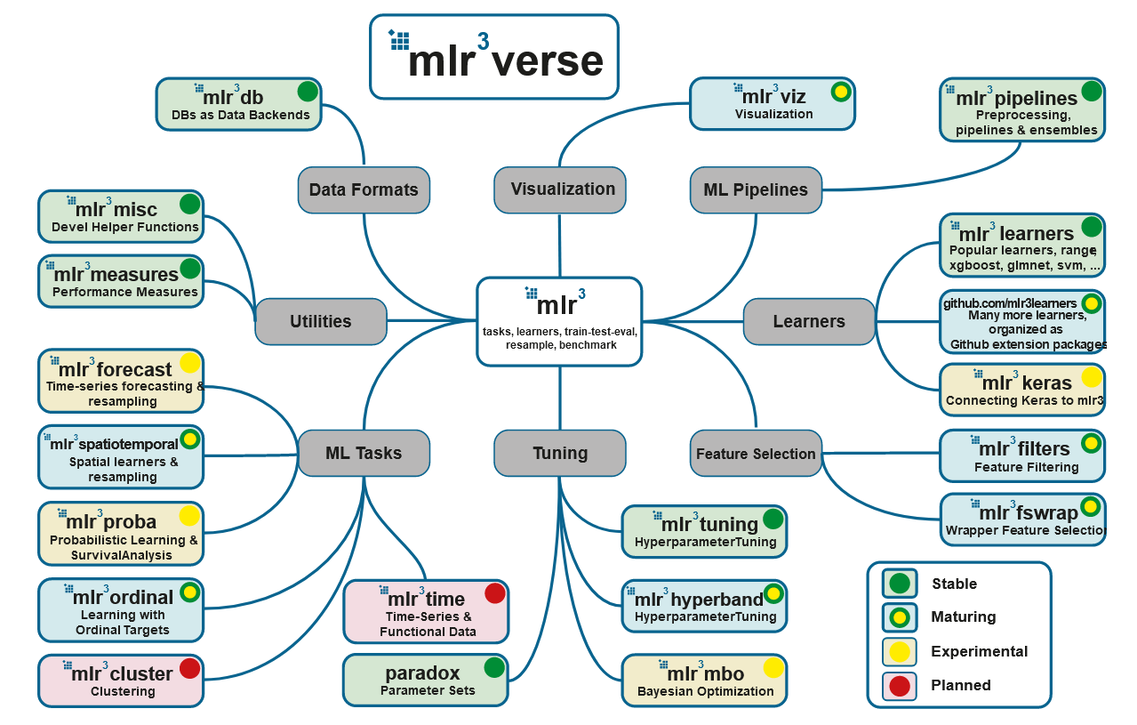
- Überblick über das Mlr3-Ökosystem
- Rohre und Diagramm der Berechnungen
1.
caret — ,
caret R ( CRAN 2007 ). 2013 Applied Predictive Modeling, .
:
- ( - );
- (-), , , ;
- , caret- - ;
- — , xgboost
nrounds, max_depth, eta, gamma, colsample_bytree, min_child_weight subsample.
:
- — , . ;
- : , . recipes , ;
- - (nested resampling), caretEnsemble.
tidyverse strikes back
tidymodels, recipes ( «» , ), rsample ( ) tune ( ).
:
- «» , ;
- , embed textrecipes;
- , . ( tune);
- workflows «» .
:
- , tune . «» , ,
apply/map-; - . , 200 ;
- - .
mlr3 vs
mlr3 mlr , caret tidymodels. mlr , mlr3.
:
- R6-, data.table;
- . , ;
- API ,
learner — ; - .
:
2. : R6- data.table
mlr3 «» , R6-. R6- , . Advanced R, , .
R6- R6Class():
library(R6)

Accumulator <- R6Class("Accumulator", list(
  sum = 0,
  add = function(x = 1) {
    self$sum <- self$sum + x
    invisible(self)
  })
)
— "Accumulator".
new(), (, , ) :
x <- Accumulator$new()
, , :
x$add(4)
x$sum
#> [1] 4
R6- :
y1 <- Accumulator$new()
y2 <- y1

y1$add(10)
c(y1 = y1$sum, y2 = y2$sum)
#> y1 y2
#> 10 10
clone() ( clone(deep = TRUE) ):
y1 <- Accumulator$new()
y2 <- y1$clone()

y1$add(10)
c(y1 = y1$sum, y2 = y2$sum)
#> y1 y2
#> 10  0
, R6 mlr3.
data.table ( , data.table data.table: R). - data.table, := . , , 2 , . , , .
3. ML- mlr3

: https://mlr3book.mlr-org.com/
mlr3 :
library(mlr3)

#
task <- TaskClassif$new(id = "iris",
                        backend = iris,
                        target = "Species")
task
# <TaskClassif:iris> (150 x 5)
# * Target: Species
# * Properties: multiclass
# * Features (4):
#   - dbl (4): Petal.Length, Petal.Width, Sepal.Length, Sepal.Width

#
# learner_rpart <- mlr_learners$get("classif.rpart")
learner_rpart <- lrn("classif.rpart",
                     predict_type = "prob",
                     minsplit = 50)
learner_rpart
# <LearnerClassifRpart:classif.rpart>
# * Model: -
# * Parameters: xval=0, minsplit=50
# * Packages: rpart
# * Predict Type: prob
# * Feature types: logical, integer, numeric, factor, ordered
# * Properties: importance, missings, multiclass, selected_features, twoclass, weights

#
learner_rpart$param_set
# ParamSet:
#                id    class lower upper levels     default value
# 1:       minsplit ParamInt     1   Inf                 20    50
# 2:      minbucket ParamInt     1   Inf        <NoDefault>
# 3:             cp ParamDbl     0     1               0.01
# 4:     maxcompete ParamInt     0   Inf                  4
# 5:   maxsurrogate ParamInt     0   Inf                  5
# 6:       maxdepth ParamInt     1    30                 30
# 7:   usesurrogate ParamInt     0     2                  2
# 8: surrogatestyle ParamInt     0     1                  0
# 9:           xval ParamInt     0   Inf                 10     0

#
learner_rpart$train(task, row_ids = 1:120)
learner_rpart$model
# n= 120
#
# node), split, n, loss, yval, (yprob)
#       * denotes terminal node
#
# 1) root 120 70 setosa (0.41666667 0.41666667 0.16666667)
#   2) Petal.Length< 2.45 50  0 setosa (1.00000000 0.00000000 0.00000000) *
#   3) Petal.Length>=2.45 70 20 versicolor (0.00000000 0.71428571 0.28571429)
#     6) Petal.Length< 4.95 49  1 versicolor (0.00000000 0.97959184 0.02040816) *
#     7) Petal.Length>=4.95 21  2 virginica (0.00000000 0.09523810 0.90476190) *
: (task) (learner).
(TaskClassif , TaskRegr ..) new(). id, backend target; positive. : mlr_tasks$get("iris") tsk("iris").
mlr_learners get() train(), task , . : lrn("classif.rpart", predict_type = "prob", minsplit = 50). (predict_type = "prob") (minsplit = 50). : learner_rpart$predict_type <- "prob", learner_rpart$param_set$values$minsplit = 50.
predict_newdata():
#
preds <- learner_rpart$predict_newdata(newdata = iris[121:150, ])
preds
# <PredictionClassif> for 30 observations:
#     row_id     truth   response prob.setosa prob.versicolor prob.virginica
#          1 virginica  virginica           0       0.0952381     0.90476190
#          2 virginica versicolor           0       0.9795918     0.02040816
#          3 virginica  virginica           0       0.0952381     0.90476190
# ---
#         28 virginica  virginica           0       0.0952381     0.90476190
#         29 virginica  virginica           0       0.0952381     0.90476190
#         30 virginica  virginica           0       0.0952381     0.90476190
- 5 :
cv10 <- rsmp("cv", folds = 5)

resample_results <- resample(task, learner_rpart, cv10)
# INFO  [09:37:05.993] Applying learner 'classif.rpart' on task 'iris' (iter 1/5)
# INFO  [09:37:06.018] Applying learner 'classif.rpart' on task 'iris' (iter 2/5)
# INFO  [09:37:06.042] Applying learner 'classif.rpart' on task 'iris' (iter 3/5)
# INFO  [09:37:06.074] Applying learner 'classif.rpart' on task 'iris' (iter 4/5)
# INFO  [09:37:06.098] Applying learner 'classif.rpart' on task 'iris' (iter 5/5)

resample_results
# <ResampleResult> of 5 iterations
# * Task: iris
# * Learner: classif.rpart
# * Warnings: 0 in 0 iterations
# * Errors: 0 in 0 iterations

#    (-):
as.data.table(mlr_resamplings)
#            key        params iters
# 1:   bootstrap repeats,ratio    30
# 2:      custom                   0
# 3:          cv         folds    10
# 4:     holdout         ratio     1
# 5: repeated_cv repeats,folds   100
# 6: subsampling repeats,ratio    30
. score() resample_results, — accuracy "classif.acc" classification error "classif.ce". , get(): mlr_measures$get("classif.ce"). msrs():
resample_results$score(msrs(c("classif.acc", "classif.ce")))[, 5:10]
#
#        resampling resampling_id iteration prediction classif.acc classif.ce
# 1: <ResamplingCV>            cv         1     <list>   0.8666667 0.13333333
# 2: <ResamplingCV>            cv         2     <list>   0.9666667 0.03333333
# 3: <ResamplingCV>            cv         3     <list>   0.9333333 0.06666667
# 4: <ResamplingCV>            cv         4     <list>   0.9666667 0.03333333
# 5: <ResamplingCV>            cv         5     <list>   0.9333333 0.06666667
4.
— . , .
. paradox:
library("paradox")
searchspace <- ParamSet$new(list(
  ParamDbl$new("cp", lower = 0.001, upper = 0.1),
  ParamInt$new("minsplit", lower = 1, upper = 10)
))
searchspace
# ParamSet:
#          id    class lower upper levels     default value
# 1:       cp ParamDbl 0.001   0.1        <NoDefault>
# 2: minsplit ParamInt 1.000  10.0        <NoDefault>
ParamSet, cp minsplit; rpart .
, searchspace . tune() Tuner. . resolution, , param_resolutions, . , , .
generate_design_grid() , :
generate_design_grid(searchspace,
                     param_resolutions = c("cp" = 2, "minsplit" = 3))
# <Design> with 6 rows:
#       cp minsplit
# 1: 0.001        1
# 2: 0.001        5
# 3: 0.001       10
# 4: 0.100        1
# 5: 0.100        5
# 6: 0.100       10
: generate_design_random() generate_design_lhs() .
, . Terminator-, , ( ), . mlr3tuning:
library("mlr3tuning")

evals20 <- term("evals", n_evals = 20)
evals20
# <TerminatorEvals>
# * Parameters: n_evals=20

#
as.data.table(mlr_terminators)
#             key
# 1:   clock_time
# 2:        combo
# 3:        evals
# 4:   model_time
# 5:         none
# 6: perf_reached
# 7:   stagnation
TuningInstance:
tuning_instance <- TuningInstance$new(
  task = TaskClassif$new(id = "iris",
                        backend = iris,
                        target = "Species"),
  learner = lrn("classif.rpart",
                predict_type = "prob"),
  resampling = rsmp("cv", folds = 5),
  measures = msr("classif.ce"),
  param_set = ParamSet$new(
    list(ParamDbl$new("cp", lower = 0.001, upper = 0.1),
         ParamInt$new("minsplit", lower = 1, upper = 10)
         )
    ),
  terminator = term("evals", n_evals = 20)
)

tuning_instance
# <TuningInstance>
# * State:  Not tuned
# * Task: <TaskClassif:iris>
# * Learner: <LearnerClassifRpart:classif.rpart>
# * Measures: classif.ce
# * Resampling: <ResamplingCV>
# * Terminator: <TerminatorEvals>
# * bm_args: list()
# * n_evals: 0
# ParamSet:
#          id    class lower upper levels     default value
# 1:       cp ParamDbl 0.001   0.1        <NoDefault>
# 2: minsplit ParamInt 1.000  10.0        <NoDefault>
— Tuner, :
tuner <- tnr("grid_search",
             resolution = 5,
             batch_size = 2)

#
# as.data.table(mlr_tuners)
#              key
# 1: design_points
# 2:         gensa
# 3:   grid_search
# 4: random_search
resolution = 5, 25 . 20 , terminator = term("evals", n_evals = 20). batch_size — , . mlr3 — , .
tnr("design_points"): , ( — , mlr3 ).
, :
result <- tuner$tune(tuning_instance)
result
# NULL
, result . , tuner$tune() tuning_instance:
tuning_instance$result
# $tune_x
# $tune_x$cp
# [1] 0.001
#
# $tune_x$minsplit
# [1] 5
#
#
# $params
# $params$xval
# [1] 0
#
# $params$cp
# [1] 0.001
#
# $params$minsplit
# [1] 5
#
#
# $perf
# classif.ce
#       0.04

result <- tuning_instance$archive(unnest = "params")
result[order(classif.ce), c("cp", "minsplit", "classif.ce")]
#         cp minsplit classif.ce
#  1: 0.00100        5 0.04000000
#  2: 0.00100        3 0.04000000
#  3: 0.00100        8 0.04000000
#  4: 0.00100        1 0.04000000
#  5: 0.00100       10 0.04666667
#  6: 0.02575       10 0.06000000
#  7: 0.07525        5 0.06000000
#  8: 0.02575        8 0.06000000
#  9: 0.02575        3 0.06000000
# 10: 0.05050        1 0.06000000
# 11: 0.07525        3 0.06000000
# 12: 0.07525        1 0.06000000
# 13: 0.05050        3 0.06000000
# 14: 0.02575        5 0.06000000
# 15: 0.05050        5 0.06000000
# 16: 0.05050        8 0.06000000
# 17: 0.10000        3 0.06000000
# 18: 0.10000        8 0.06000000
# 19: 0.05050       10 0.06000000
# 20: 0.10000        1 0.06000000

library(ggplot2)
ggplot(result,
       aes(x = cp, y = classif.ce, color = as.factor(minsplit))) +
  geom_line() +
  geom_point(size = 3)

, tune():
Tuner ( batch_size);Learner Task . ResampleResult ( BenchmarkResult);Terminator , . , 1, , ;- ;
- , ( , ,
msr("classif.ce", aggregator = "median").
tuning_instance$bmr, BenchmarkResult, score() as.data.table(tuning_instance$bmr). , , ResampleResult tuning_instance$archive():
tuning_instance$archive()[1, resample_result][[1]]$score()[, 4:9]
#       learner_id     resampling resampling_id iteration prediction classif.ce
# 1: classif.rpart <ResamplingCV>            cv         1     <list> 0.06666667
# 2: classif.rpart <ResamplingCV>            cv         2     <list> 0.16666667
# 3: classif.rpart <ResamplingCV>            cv         3     <list> 0.03333333
# 4: classif.rpart <ResamplingCV>            cv         4     <list> 0.03333333
# 5: classif.rpart <ResamplingCV>            cv         5     <list> 0.00000000
, :
res <- tuning_instance$archive(unnest = "params")
res[, ce_resemples := lapply(resample_result, function(x) x$score()[, classif.ce])]
ce_resemples <- res[, .(ce_resemples = unlist(ce_resemples)), by = nr]
res[ce_resemples, on = "nr"]
5. mlr3
: mlr3, mlr3tuning paradox. , - mlr3verse:
# install.packages("mlr3verse")
library(mlr3verse)
## Loading required package: mlr3
## Loading required package: mlr3db
## Loading required package: mlr3filters
## Loading required package: mlr3learners
## Loading required package: mlr3pipelines
## Loading required package: mlr3tuning
## Loading required package: mlr3viz
## Loading required package: paradox
- mlr3db dbplyr data.table.
- mlr3filters , ( ).
- mlr3learners (
regr.glmnet, regr.kknn, regr.km, regr.lm, regr.ranger, regr.svm, regr.xgboost) (classif.glmnet, classif.kknn, classif.lda, classif.log_reg, classif.multinom, classif.naive_bayes, classif.qda, classif.ranger, classif.svm, classif.xgboost). . - mlr3pipelines (pipelines), . , , CRAN, :
remotes::install_github("https://github.com/mlr-org/mlr3pipelines"). - mlr3tuning .
- mlr3viz , .
- mlr3measures — ~40 . mlr3verse , .
, .
6.
(pipelines) , , .
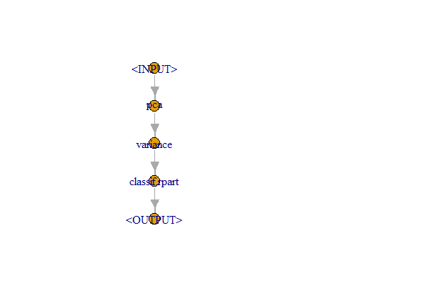
— , , — . PipeOpLearner(), — PipeOpFilter(), — PipeOp(). ( po()) :
pca <- po("pca")
filter <- po("filter",
             filter = mlr3filters::flt("variance"),
             filter.frac = 0.5)
learner_po <- po("learner",
                 learner = lrn("classif.rpart"))
%>>%:
graph <- pca %>>% filter %>>% learner_po
graph$plot()
. , :
gr <- Graph$new()$
  add_pipeop(mlr_pipeops$get("copy", outnum = 2))$
  add_pipeop(mlr_pipeops$get("scale"))$
  add_pipeop(mlr_pipeops$get("pca"))$
  add_pipeop(mlr_pipeops$get("featureunion", innum = 2))

gr$
  add_edge("copy", "scale", src_channel = 1)$
  add_edge("copy", "pca", src_channel = "output2")$
  add_edge("scale", "featureunion", dst_channel = 1)$
  add_edge("pca", "featureunion", dst_channel = 2)

gr$plot(html = FALSE)

, (po("learner", learner = lrn("classif.rpart"))). , :
glrn <- GraphLearner$new(graph)
glrn
# <GraphLearner:pca.variance.classif.rpart>
# * Model: -
# * Parameters: variance.filter.frac=0.5, variance.na.rm=TRUE, classif.rpart.xval=0
# * Packages: -
# * Predict Type: response
# * Feature types: logical, integer, numeric, character, factor, ordered, POSIXct
# * Properties: importance, missings, multiclass, oob_error, selected_features, twoclass,
#   weights
GraphLearner Learner. , Learner-, :
resample(tsk("iris"), glrn, rsmp("cv"))
# INFO  [17:17:00.358] Applying learner 'pca.variance.classif.rpart' on task 'iris' (iter 1/10)
# INFO  [17:17:00.615] Applying learner 'pca.variance.classif.rpart' on task 'iris' (iter 2/10)
# INFO  [17:17:00.881] Applying learner 'pca.variance.classif.rpart' on task 'iris' (iter 3/10)
# INFO  [17:17:01.087] Applying learner 'pca.variance.classif.rpart' on task 'iris' (iter 4/10)
# INFO  [17:17:01.303] Applying learner 'pca.variance.classif.rpart' on task 'iris' (iter 5/10)
# INFO  [17:17:01.518] Applying learner 'pca.variance.classif.rpart' on task 'iris' (iter 6/10)
# INFO  [17:17:01.716] Applying learner 'pca.variance.classif.rpart' on task 'iris' (iter 7/10)
# INFO  [17:17:01.927] Applying learner 'pca.variance.classif.rpart' on task 'iris' (iter 8/10)
# INFO  [17:17:02.129] Applying learner 'pca.variance.classif.rpart' on task 'iris' (iter 9/10)
# INFO  [17:17:02.337] Applying learner 'pca.variance.classif.rpart' on task 'iris' (iter 10/10)
# <ResampleResult> of 10 iterations
# * Task: iris
# * Learner: pca.variance.classif.rpart
# * Warnings: 0 in 0 iterations
# * Errors: 0 in 0 iterations
, issue How to deal with different preprocessing steps as hyperparameters:
gr <- pipeline_branch(list(pca = po("pca"), nothing = po("nop")))
gr$plot()

caret tidymodels !
, mlr3. mlr3 book .