أي نشاط يولد البيانات. أياً كان ما تفعله ، فمن المحتمل أن يكون لديك بين يديك مخزن من المعلومات المفيدة الخام ، أو على الأقل الوصول إلى مصدره.
اليوم الفائز هو الذي يتخذ القرارات بناءً على بيانات موضوعية. أصبحت مهارات المحلل أكثر ملاءمة من أي وقت مضى ، وتوافر الأدوات اللازمة في متناول يدك يسمح لك دائمًا أن تكون متقدمًا بخطوة. هذه مساعدة في ظهور هذه المقالة.
هل لديك عملك الخاص؟ أو ربما ... على الرغم من ذلك ، لا يهم. عملية استخراج البيانات لا نهاية لها ومثيرة. وحتى مجرد البحث بشكل جيد على الإنترنت ، يمكنك العثور على مجال للنشاط.
إليك ما لدينا اليوم - قاعدة بيانات توزيع XML غير رسمية لـ RuTracker.ORG. يتم تحديث قاعدة البيانات كل ستة أشهر وتحتوي على معلومات حول جميع التوزيعات لتاريخ وجود هذا تعقب سيل.
ماذا يمكن أن تخبر أصحاب rutracker؟ والمتواطئون المباشرون للقرصنة على الإنترنت؟ أو مستخدم عادي مغرم أنيمي ، على سبيل المثال؟
هل تفهم ما أقصد؟
المكدس - R ، Clickhouse ، Dataiku
تمر أي تحليلات بعدة مراحل رئيسية: استخراج البيانات وإعدادها ودراسة البيانات (التصور). كل مرحلة لها أداتها الخاصة. لأن مكدس اليوم:
- ر. نعم ، لا يحظى بشعبية ويقل عن بايثون. ولكن لا تزال نظيفة وجميلة مع dplyr و ggplot2. ولد للتحليلات وعدم استخدامه جريمة.
- كليك هاوس. عمود DBMS التحليلي. سمعت بالتأكيد: "كليكهاوس لا يبطئ" أو "سرعة على حافة الخيال". الناس لا يكذبون وسنرى ذلك. المسؤول عن اللحظية.
- Dataiku. منصة لمعالجة وتصور وتحليل الأعمال التنبؤية.
مراجعة: يعمل Dataiku على Linux و Mac. يتوفر إصدار مجاني بحد أقصى للمستخدمين 3 أشخاص. الوثائق هنا .
والمثير للدهشة أنه لا يوجد حتى الآن ضجيج أو ضجيج ، إذا كنت ترغب ، في عدم قابلية هذه المنصة للمقاومة على موارد اللغة الروسية وحتى على حبري. سآخذ لتصحيح سوء الفهم هذا وأطلب منك تهنئة dataiku على المبادرة.
البيانات الضخمة - مشاكل كبيرة
xml– 5 . – rutracker.org, (2005 .) 2019 . 15 !
R Studio – ! . , .
, R. Big Data, Clickhouse … , xml–. . .
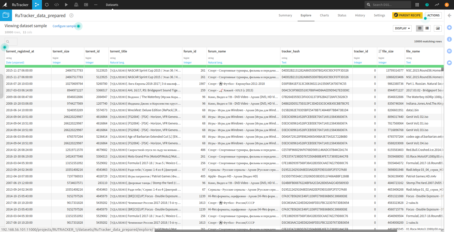
. Dataiku DSS . – 10 000 . . , . , 200 000 .
, . .

. : content — json.
content, . – .
recipe — . , . json .
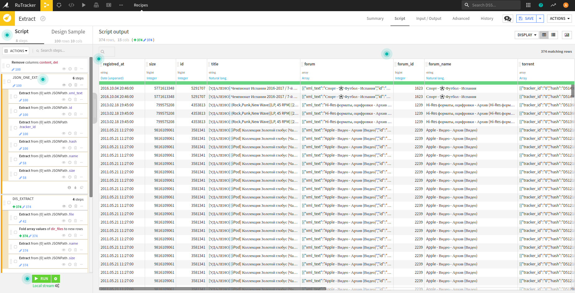
. , , + dataiku.
recipe, — .
csv Clickhouse.
Clickhouse 15 rutracker-a.
?
SELECT ROUND(uniq(torrent_id) / 1000000, 2) AS Count_M
FROM rutracker

┌─Count_M─┐
│    1.46 │
└─────────┘
1 rows in set. Elapsed: 0.247 sec. Processed 25.51 million rows, 204.06 MB (103.47 million rows/s., 827.77 MB/s.)
1.5 25 . 0.3 ! .
, , .
SELECT COUNT(*) AS Count
FROM rutracker
WHERE (file_ext = 'epub') OR (file_ext = 'fb2') OR (file_ext = 'mobi')

┌──Count─┐
│ 333654 │
└────────┘
1 rows in set. Elapsed: 0.435 sec. Processed 25.51 million rows, 308.79 MB (58.64 million rows/s., 709.86 MB/s.)
300 — ! , . .
SELECT ROUND(SUM(file_size) / 1000000000, 2) AS Total_size_GB
FROM rutracker
WHERE (file_ext = 'epub') OR (file_ext = 'fb2') OR (file_ext = 'mobi')

┌─Total_size_GB─┐
│        625.75 │
└───────────────┘
1 rows in set. Elapsed: 0.296 sec. Processed 25.51 million rows, 344.32 MB (86.24 million rows/s., 1.16 GB/s.)
– 25 . , ?
R
R. , DBI ( ). Clickhouse.
Rlibrary(DBI) # , ... Clickhouse
library(dplyr) # %>%
#
library(ggplot2)
library(ggrepel)
library(cowplot)
library(scales)
library(ggrepel)
# localhost:9000
connection <- dbConnect(RClickhouse::clickhouse(), host="localhost", port = 9000)
, . dplyr .
? rutracker.org .
Ryears_stat <- dbGetQuery(connection,
"SELECT
round(COUNT(*)/1000000, 2) AS Files,
round(uniq(torrent_id)/1000, 2) AS Torrents,
toYear(torrent_registred_at) AS Year
FROM rutracker
GROUP BY Year")
ggplot(years_stat, aes(as.factor(Year), as.double(Files))) +
geom_bar(stat = 'identity', fill = "darkblue", alpha = 0.8)+
theme_minimal() +
labs(title = " RuTracker", subtitle = " 2005 - 2019\n")+
theme(axis.text.x = element_text(angle=90, vjust = 0.5),
axis.text.y = element_text(),
axis.title.y = element_blank(),
axis.title.x = element_blank(),
panel.grid.major.x = element_blank(),
panel.grid.major.y = element_line(size = 0.9),
panel.grid.minor.y = element_line(size = 0.4),
plot.title = element_text(vjust = 3, hjust = 0, family = "sans", size = 16, color = "#101010", face = "bold"),
plot.caption = element_text(vjust = 3, hjust = 0, family = "sans", size = 12, color = "#101010", face = "bold"),
plot.margin = unit(c(1,0.5,1,0.5), "cm"))+
scale_y_continuous(labels = number_format(accuracy = 1, suffix = " "))
ggplot(years_stat, aes(as.factor(Year), as.integer(Torrents))) +
geom_bar(stat = 'identity', fill = "#008b8b", alpha = 0.8)+
theme_minimal() +
labs(title = " RuTracker", subtitle = " 2005 - 2019\n", caption = "* ")+
theme(axis.text.x = element_text(angle=90, vjust = 0.5),
axis.text.y = element_text(),
axis.title.y = element_blank(),
axis.title.x = element_blank(),
panel.grid.major.x = element_blank(),
panel.grid.major.y = element_line(size = 0.9),
panel.grid.minor.y = element_line(size = 0.4),
plot.title = element_text(vjust = 3, hjust = 0, family = "sans", size = 16, color = "#101010", face = "bold"),
plot.caption = element_text(vjust = -3, hjust = 1, family = "sans", size = 9, color = "grey60", face = "plain"),
plot.margin = unit(c(1,0.5,1,0.5), "cm")) +
scale_y_continuous(labels = number_format(accuracy = 1, suffix = " "))
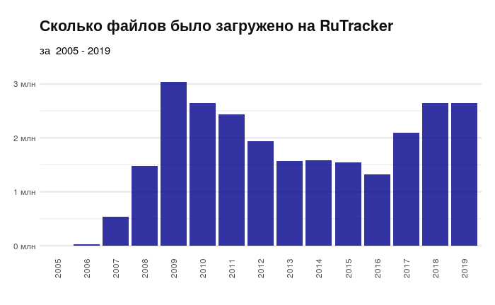
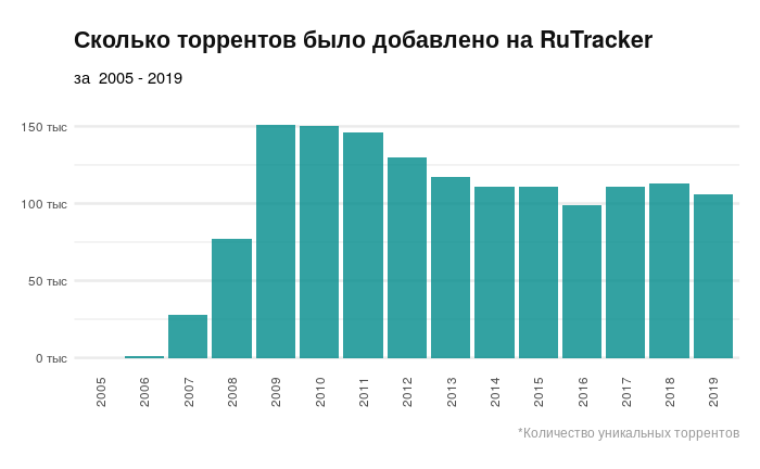
2016 . , 2016 rutracker.org . , .
, . , .
.
Rextention_stat <- dbGetQuery(connection,
"SELECT toYear(torrent_registred_at) AS Year,
COUNT(tracker_id)/1000 AS Count,
ROUND(SUM(file_size)/1000000000000, 2) AS Total_Size_TB,
file_ext
FROM rutracker
GROUP BY Year, file_ext
ORDER BY Year, Count")
#
TopExt <- function(x, n) {
res_tab <- NULL
# 2005 2006, ..
for (i in (3:15)) {
res_tab <-bind_rows(list(res_tab,
extention_stat %>% filter(Year == x[i]) %>%
arrange(desc(Count), desc(Total_Size_TB)) %>%
head(n)
))
}
return(res_tab)
}
years_list <- unique(extention_stat$Year)
ext_data <- TopExt(years_list, 5)
ggplot(ext_data, aes(as.factor(Year), as.integer(Count), fill = file_ext)) +
geom_bar(stat = "identity",position="dodge2", alpha =0.8, width = 1)+
theme_minimal() +
labs(title = " RuTracker",
subtitle = " 2005 - 2019\n",
caption = "* -5 ", fill = "") +
theme(axis.text.x = element_text(angle=90, vjust = 0.5),
axis.text.y = element_text(),
axis.title.y = element_blank(),
axis.title.x = element_blank(),
panel.grid.major.x = element_blank(),
panel.grid.major.y = element_line(size = 0.9),
panel.grid.minor.y = element_line(size = 0.4),
legend.title = element_text(vjust = 1, hjust = -1, family = "sans", size = 9, color = "#101010", face = "plain"),
legend.position = "top",
plot.title = element_text(vjust = 3, hjust = 0, family = "sans", size = 16, color = "#101010", face = "bold"),
plot.caption = element_text(vjust = -4, hjust = 1, family = "sans", size = 9, color = "grey60", face = "plain"),
plot.margin = unit(c(1,0.5,1,0.5), "cm")) +
scale_y_continuous(labels = number_format(accuracy = 0.5, scale = (1/1000), suffix = " "))+guides(fill=guide_legend(nrow=1))
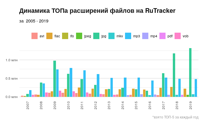
. . .
rutracker-a. .
Rchapter_stat <- dbGetQuery(connection,
"SELECT
substring(forum_name, 1, position(forum_name, ' -')) Chapter,
uniq(torrent_id) AS Count,
ROUND(median(file_size)/1000000, 2) AS Median_Size_MB,
ROUND(max(file_size)/1000000000) AS Max_Size_GB,
ROUND(SUM(file_size)/1000000000000) AS Total_Size_TB
FROM rutracker WHERE Chapter NOT LIKE('\"%')
GROUP BY Chapter
ORDER BY Count DESC")
chapter_stat$Count <- as.integer(chapter_stat$Count)
#
AggChapter2 <- function(Chapter){
var_ch <- str(Chapter)
res = NULL
for(i in (1:22)){
select_str <-paste0(
"SELECT
toYear(torrent_registred_at) AS Year,
substring(forum_name, 1, position(forum_name, ' -')) Chapter,
uniq(torrent_id)/1000 AS Count,
ROUND(median(file_size)/1000000, 2) AS Median_Size_MB,
ROUND(max(file_size)/1000000000,2) AS Max_Size_GB,
ROUND(SUM(file_size)/1000000000000,2) AS Total_Size_TB
FROM rutracker
WHERE Chapter LIKE('", Chapter[i], "%')
GROUP BY Year, Chapter
ORDER BY Year")
res <-bind_rows(list(res, dbGetQuery(connection, select_str)))
}
return(res)
}
chapters_data <- AggChapter2(chapter_stat$Chapter)
chapters_data$Chapter <- as.factor(chapters_data$Chapter)
chapters_data$Count <- as.numeric(chapters_data$Count)
chapters_data %>% group_by(Chapter)%>%
ggplot(mapping = aes(x = reorder(Chapter, Total_Size_TB), y = Total_Size_TB))+
geom_bar(stat = "identity", fill="darkblue", alpha =0.8)+
theme(panel.grid.major.x = element_line(colour="grey60", linetype="dashed"))+
xlab('\n') + theme_minimal() +
labs(title = "C RuTracker-",
subtitle = " 2019\n")+
theme(axis.text.x = element_text(),
axis.text.y = element_text(family = "sans", size = 9, color = "#101010", hjust = 1, vjust = 0.5),
axis.title.y = element_text(vjust = 2.5, hjust = 0, family = "sans", size = 9, color = "grey40", face = "plain"),
axis.title.x = element_blank(),
axis.line.x = element_line(color = "grey60", size = 0.1, linetype = "solid"),
panel.grid.major.y = element_blank(),
panel.grid.major.x = element_line(size = 0.7, linetype = "solid"),
panel.grid.minor.x = element_line(size = 0.4, linetype = "solid"),
plot.title = element_text(vjust = 3, hjust = 1, family = "sans", size = 16, color = "#101010", face = "bold"),
plot.subtitle = element_text(vjust = 2, hjust = 1, family = "sans", size = 12, color = "#101010", face = "plain"),
plot.caption = element_text(vjust = -3, hjust = 1, family = "sans", size = 9, color = "grey60", face = "plain"),
plot.margin = unit(c(1,0.5,1,0.5), "cm"))+
scale_y_continuous(labels = number_format(accuracy = 1, suffix = " "))+
coord_flip()
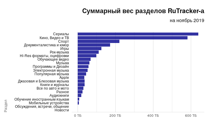
. — — . , . , Apple.
Rchapters_data %>% group_by(Chapter)%>%
ggplot(mapping = aes(x = reorder(Chapter, Count), y = Count))+
geom_bar(stat = "identity", fill="#008b8b", alpha =0.8)+
theme(panel.grid.major.x = element_line(colour="grey60", linetype="dashed"))+
xlab('') + theme_minimal() +
labs(title = " RuTracker-",
subtitle = " 2019\n")+
theme(axis.text.x = element_text(),
axis.text.y = element_text(family = "sans", size = 9, color = "#101010", hjust = 1, vjust = 0.5),
axis.title.y = element_text(vjust = 3.5, hjust = 0, family = "sans", size = 9, color = "grey40", face = "plain"),
axis.title.x = element_blank(),
axis.line.x = element_line(color = "grey60", size = 0.1, linetype = "solid"),
panel.grid.major.y = element_blank(),
panel.grid.major.x = element_line(size = 0.7, linetype = "solid"),
panel.grid.minor.x = element_line(size = 0.4, linetype = "solid"),
plot.title = element_text(vjust = 3, hjust = 1, family = "sans", size = 16, color = "#101010", face = "bold"),
plot.subtitle = element_text(vjust = 2, hjust = 1, family = "sans", size = 12, color = "#101010", face = "plain"),
plot.caption = element_text(vjust = -3, hjust = 1, family = "sans", size = 9, color = "grey60", face = "plain"),
plot.margin = unit(c(1,0.5,1,0.5), "cm"))+
scale_y_continuous(limits = c(0, 300), labels = number_format(accuracy = 1, suffix = " "))+
coord_flip()
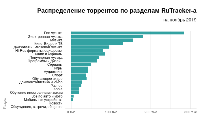
, , : -.
~15 .
Rlibrary("RColorBrewer")
getPalette = colorRampPalette(brewer.pal(19, "Spectral"))
chapters_data %>% #filter(Chapter %in% chapter_stat$Chapter[c(4,6,7,9:20)])%>%
filter(!Chapter %in% chapter_stat$Chapter[c(16, 21, 22)])%>%
filter(Year>=2007)%>%
ggplot(mapping = aes(x = Year, y = Count, fill = as.factor(Chapter)))+
geom_area(alpha =0.8, position = "fill")+
theme_minimal() +
labs(title = " -",
subtitle = " ~15 ", fill = "")+
theme(axis.text.x = element_text(vjust = 0.5),
axis.text.y = element_blank(),
axis.title.y = element_blank(),
axis.title.x = element_blank(),
panel.grid.major.x = element_blank(),
panel.grid.major.y = element_line(size = 0.9),
panel.grid.minor.y = element_line(size = 0.4),
plot.title = element_text(vjust = 3, hjust = 0, family = "sans", size = 16, color = "#101010", face = "bold"),
plot.caption = element_text(vjust = -3, hjust = 1, family = "sans", size = 9, color = "grey60", face = "plain"),
plot.margin = unit(c(1,1,1,1), "cm")) +
scale_x_continuous(breaks = c(2008, 2010, 2012, 2014, 2016, 2018),expand=c(0,0)) +
scale_fill_manual(values = getPalette(19))
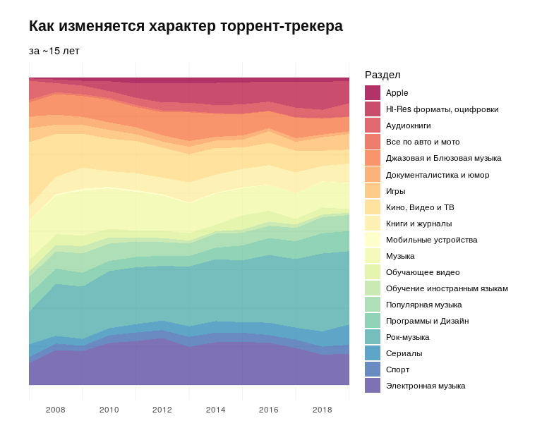
- — . — Apple , .
. .
, Rutracker-a. - rutracker.org.
Runique_torr_per_day <- dbGetQuery(connection,
"SELECT toDate(torrent_registred_at) AS date,
uniq(torrent_id) AS count
FROM rutracker
GROUP BY date
ORDER BY date")
unique_torr_per_day %>%
ggplot(aes(format(date, "%Y"), format(date, "%j"), fill = as.numeric(count)))+
geom_tile() +
theme_minimal() +
labs(title = " RuTracker-a",
subtitle = " ~15 \n\n",
fill = "- \n")+
theme(axis.text.x = element_text(vjust = 0.5),
axis.text.y = element_text(),
axis.title.y = element_blank(),
axis.title.x = element_blank(),
panel.grid.major.y = element_blank(),
panel.grid.major.x = element_line(size = 0.9),
panel.grid.minor.x = element_line(size = 0.4),
legend.title = element_text(vjust = 0.7, hjust = -1, family = "sans", size = 10, color = "#101010", face = "plain"),
legend.position = c(0.88, 1.30),
legend.direction = "horizontal",
plot.title = element_text(vjust = 3, hjust = 0, family = "sans", size = 16, color = "#101010", face = "bold"),
plot.caption = element_text(vjust = -3, hjust = 1, family = "sans", size = 9, color = "grey60", face = "plain"),
plot.margin = unit(c(1,1,1,1), "cm"))+ coord_flip(clip = "off") +
scale_y_discrete(breaks = c(format(as.Date("2007-01-15"), "%j"),
format(as.Date("2007-02-15"), "%j"),
format(as.Date("2007-03-15"), "%j"),
format(as.Date("2007-04-15"), "%j"),
format(as.Date("2007-05-15"), "%j"),
format(as.Date("2007-06-15"), "%j"),
format(as.Date("2007-07-15"), "%j"),
format(as.Date("2007-08-15"), "%j"),
format(as.Date("2007-09-15"), "%j"),
format(as.Date("2007-10-15"), "%j"),
format(as.Date("2007-11-15"), "%j"),
format(as.Date("2007-12-15"), "%j")),
labels = c("", "", "", "", "", "","", "", "", "","",""), position = 'right') +
scale_fill_gradientn(colours = c("#155220", "#c6e48b")) +
annotate(geom = "curve", x = 16.5, y = 119, xend = 13, yend = 135,
curvature = .3, color = "grey15", arrow = arrow(length = unit(2, "mm"))) +
annotate(geom = "text", x = 16, y = 45,
label = " « » \n",
hjust = "left", vjust = -0.75, color = "grey25") +
guides(x.sec = guide_axis_label_trans(~.x)) +
annotate("rect", xmin = 11.5, xmax = 12.5, ymin = 1, ymax = 366,
alpha = .0, colour = "white", size = 0.1) +
geom_segment(aes(x = 11.5, y = 25, xend = 12.5, yend = 25, colour = "segment"),
show.legend = FALSE)
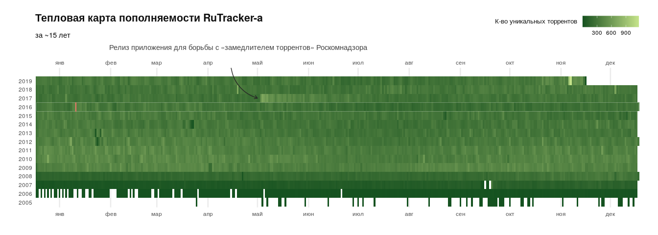
2017 . (. GitHub ). 2016 , . .
. . – .
, content , , , 15 .
Dataiku
, : , , , .
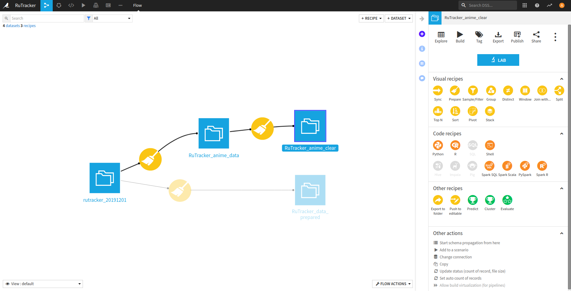
, -. . – .
– .
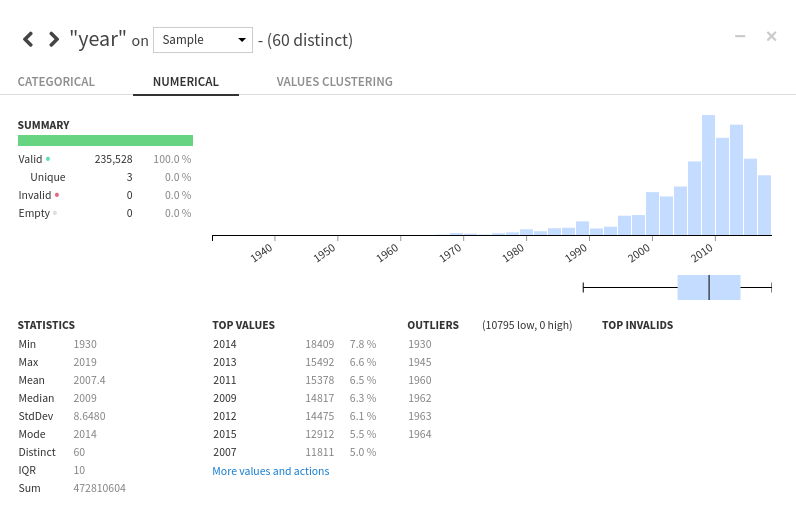
: rutracker.org , , — 60. 2009 — 2014 .
. , , . .
, . .

, dataiku — . , , (R, Python), . .
, RuTracker, : , . . , . .
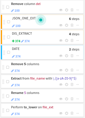
UPD: , recipe dataiku.
بشكل مشروط ، يمكن تقسيم الوصفة الواردة في هذه المقالة إلى قسمين: إعداد البيانات للتحليل في R وإعداد البيانات حول الأنيمي للتحليل مباشرة على النظام الأساسي.
مرحلة التحضير للتحليل في Rjson- .
json-. .
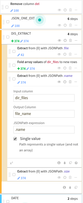
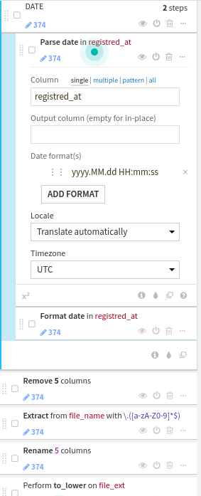
timestamp .
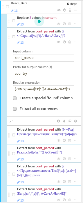
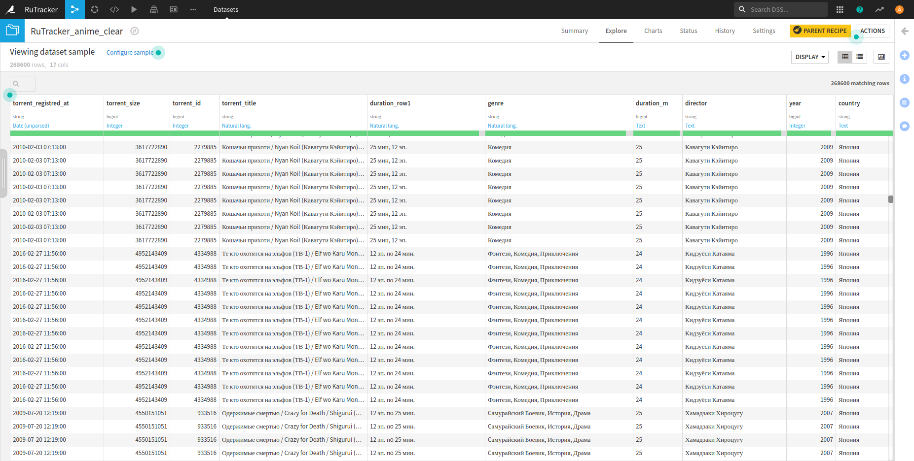
مرحلة إعداد بيانات الأنمي, , . content — Descr_Data.
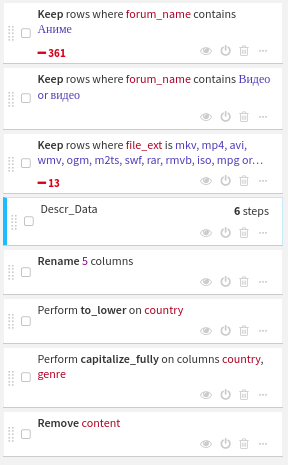
contentregexp , , , . , regexp dataiku .