تحليل شعبية مقاطع فيديو يوتيوب للمشاركين في يوروفيجن 2020

في 13 مارس ، على قناة يوروفيجن الرسمية على يوتيوب ، تم نشر تشكيل مجموعة Little Big ، والتي ستمثل روسيا في المسابقة. بعد مشاهدة المقطع ، أردت مقارنة إحصائيات فيديو مجموعتنا بمقاطع الفيديو الخاصة بالمشاركين الآخرين ؛ مقاطع الفيديو الأكثر مشاهدة ، والتي لديها أعلى نسبة من الإعجابات ، والتي يتم التعليق عليها غالبًا. جوجل الإحصائيات النهائية لم يؤد إلى أي شيء. لذلك تقرر جمع الإحصائيات اللازمة.

هيكل المقالة:

• رمز التحميل
• تحليل
• تحديث بتاريخ 03/14/2020 20:30
• بالإضافة إلى ذلك: ننظر إلى اعتماد وجهات النظر على سكان البلاد

من خلال فتح قائمة تشغيل المشاركين ، يمكنك مشاهدة 39 مقطع فيديو ، في الواقع هناك 38 أغنية ، تكوين الإعصار - Hasta La Vista - صربيا تم تنزيله مرتين ، لذلك سيتم تلخيص الإحصائيات الموجودة عليه. لجمع الإحصائيات ، سنستخدم R.

رمز التحميل

سنحتاج إلى الحزم التالية:

library(tuber) #    API YouTube,     
library(dplyr) #     
library(ggplot2) #  

أولاً ، انتقل إلى وحدة تحكم مطوّري برامج Google وأنشئ مفتاح OAuth على واجهة برمجة تطبيقات YouTube Data API v3. بعد استلام المفتاح ، قم بتسجيل الدخول من R.

yt_oauth(" ", "  ")

الآن يمكننا جمع الإحصائيات:

#     
list_videos <- get_playlist_items(filter = c(playlist_id = "PLmWYEDTNOGUL69D2wj9m2onBKV2s3uT5Y"))

#    ,  get_stats
stats_videos <- lapply(as.character(list_videos$contentDetails.videoId), get_stats) %>% 
  bind_rows()
stats_videos <- stats_videos %>% 
  mutate_at(vars(-id), as.integer)

#   ,  get_video_details
description_videos <- lapply(as.character(list_videos$contentDetails.videoId), get_video_details)
description_videos <- lapply(description_videos, function(x) {
    list(
      id = x[["items"]][[1]][["id"]],
      name_video = x[["items"]][[1]][["snippet"]][["title"]]
    )
  }) %>% 
  bind_rows()

.. — — [ ] — Official Music Video — Eurovision 2020, , . .

#     
description_videos$name_video <- description_videos$name_video %>% 
  gsub("[^[:alnum:][:blank:]?&/\\-]", '', .) %>% 
  gsub("(  .*)|( - Offic.*)", '', .)

#      
df <- description_videos %>% 
  left_join(stats_videos, by = 'id') %>% 
  rowwise() %>% 
  mutate( #   
    proc_like = round(likeCount / (likeCount + dislikeCount), 2)
    ) %>% 
  ungroup()

# Hurricane - Hasta La Vista - Serbia     ,  
df <- df %>% 
  group_by(name_video) %>% 
  summarise(
    id = first(id),
    viewCount = sum(viewCount),
    likeCount = sum(likeCount),
    dislikeCount = sum(dislikeCount),
    commentCount = sum(commentCount),
    proc_like = round(likeCount / (likeCount + dislikeCount), 2)
  )

df$color <- ifelse(df$name_video == 'Little Big - Uno - Russia','red','gray')

. .

# - 
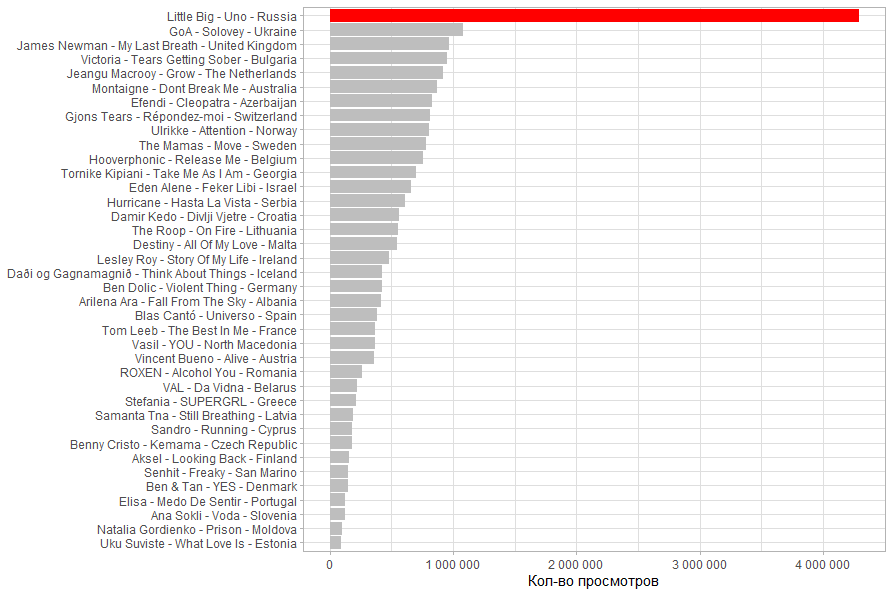
ggplot(df, aes(x = reorder(name_video, viewCount), y = viewCount, fill = color)) +
  geom_col() +
  coord_flip() +
  theme_light() +
  labs(x = NULL, y = "- ") +
  guides(fill = F) +
  scale_fill_manual(values = c('gray', 'red')) +
  scale_y_continuous(labels = scales::number_format(big.mark = " "))

#    
ggplot(df, aes(x = reorder(name_video, proc_like), y = proc_like, fill = color)) +
  geom_col() +
  coord_flip() +
  theme_light() +
  labs(x = NULL, y = "   ") +
  guides(fill = F) +
  scale_fill_manual(values = c('gray', 'red')) +
  scale_y_continuous(labels = scales::percent_format(accuracy = 1))

# - 
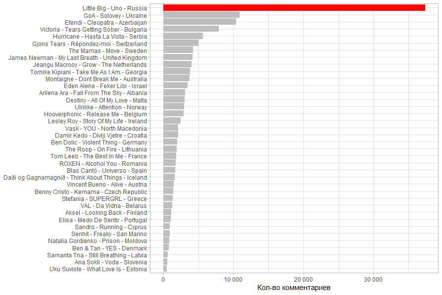
ggplot(df, aes(x = reorder(name_video, commentCount), y = commentCount, fill = color)) +
  geom_col() +
  coord_flip() +
  theme_light() +
  labs(x = NULL, y = "- ") +
  guides(fill = F) +
  scale_fill_manual(values = c('gray', 'red')) +
  scale_y_continuous(labels = scales::number_format(big.mark = " "))

#    
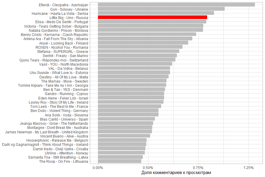
ggplot(df, aes(x = reorder(name_video, commentCount/viewCount), y = commentCount/viewCount, fill = color)) +
  geom_col() +
  coord_flip() +
  theme_light() +
  labs(x = NULL, y = "   ") +
  guides(fill = F) +
  scale_fill_manual(values = c('gray', 'red')) +
  scale_y_continuous(labels = scales::percent_format(accuracy = 0.25))

, Little Big 1 , .

. Little Big , . - .

, . . .

.

( / ). . .

13.03.2020 18:00 , , , .

UPD: 14.03.2020 20:30

. . Little Big , .

, . Little Big ,

.

( / ). 2 , , , . .

14.03.2020 20:30 , , , , . .

:

helg1978 . .

library(rvest)
library(tidyr)

#   
hdoc <- read_html('https://en.wikipedia.org/wiki/List_of_countries_and_dependencies_by_population')

tnode <- html_node(hdoc, xpath = '/html/body/div[3]/div[3]/div[4]/div/table')
df_population <- html_table(tnode)

df_population <- df_population %>% filter(`Country (or dependent territory)` != 'World')

df_population$Population <- as.integer(gsub(',','',df_population$Population,fixed = T))

df_population$`Country (or dependent territory)` <- gsub('\\[.*\\]','', df_population$`Country (or dependent territory)`)

df_population <- df_population %>% 
  select(
    `Country (or dependent territory)`,
    Population
    ) %>% 
  rename(Country = `Country (or dependent territory)`)

#       
df2 <- df %>% 
  separate(name_video, c('compozitor', 'name_track', 'Country'), ' - ', remove = F) %>% 
  mutate(Country = ifelse(Country == 'The Netherlands', 'Netherlands', Country)) %>% 
  left_join(df_population, by = 'Country')

#     
cor(df2$viewCount,df2$Population)
ggplot(df2, aes(x = Population, y =  viewCount)) +
  geom_point() +
  theme_light() +
  geom_smooth(method = 'lm') +
  labs(x = ", ", y = "- ") +
  scale_y_continuous(labels = scales::number_format(big.mark = " ")) +
  scale_x_continuous(labels = scales::number_format(big.mark = " "))

#     ,  
cor(df2[df2$Country != 'Russia',]$viewCount,df2[df2$Country != 'Russia',]$Population)
ggplot(df2 %>% filter(Country != 'Russia') , aes(x = Population, y = viewCount)) +
  geom_point() +
  theme_light() +
  geom_smooth(method = 'lm') +
  labs(x = ", ", y = "- ") +
  scale_y_continuous(labels = scales::number_format(big.mark = " ")) +
  scale_x_continuous(labels = scales::number_format(big.mark = " "))

#     , 
cor(df2$viewCount,df2$Population, method = "spearman")
ggplot(df2 , aes(x = rank(Population), y = rank(viewCount))) +
  geom_point() +
  theme_light() +
  geom_smooth(method = 'lm') +
  labs(x = ",  (  1  40)", y = "-  (  1  40)") +
  guides(fill = F)

#     
ggplot(df2, aes(x = reorder(name_video, viewCount/Population), y = viewCount/Population, fill = color)) +
  geom_col() +
  coord_flip() +
  theme_light() +
  labs(x = NULL, y = "    ") +
  guides(fill = F) +
  scale_fill_manual(values = c('gray', 'red')) +
  scale_y_continuous(labels = scales::percent_format(accuracy = 0.25))

, , 50 . 71%.

. 71% 15%. .

( ), , (. . 40%).

وكمرجع قمت بحساب نسبة المشاهدات من سكان البلاد. بالنسبة للدول الصغيرة على وجه الخصوص ، اتضح أنه تمت مراقبتها أكثر من دول أخرى. على وجه الخصوص ، هي مالطا وسان مارينو وأيسلندا.

كود جيثب الكامل