⚖️ 🎖️ 🐈 Python Anomaly Detection باستخدام Autoencoders في Python 🌉 🙏🏻 👩🏾‍🤝‍👨🏿

يعد اكتشاف الشذوذ مهمة مهمة للتعلم الآلي. لا توجد طريقة محددة لحلها ، لأن كل مجموعة بيانات لها خصائصها الخاصة. ولكن في نفس الوقت ، هناك العديد من الأساليب التي تساعد على النجاح. أريد أن أتحدث عن أحد هذه الأساليب - ترميز السيارات.

أي مجموعة بيانات تختار؟

القضية الأكثر إلحاحًا في حياة أي عالم بيانات. لتبسيط القصة ، سأستخدم مجموعة بيانات بسيطة في الهيكل ، والتي سننشئها هنا.

#  
import os
import numpy as np
from sklearn.model_selection import train_test_split
import matplotlib.pyplot as plt
from matplotlib.colors import Normalize

#        
def gen_normal_distribution(mu, sigma, size, range=(0, 1), max_val=1):
  bins = np.linspace(*range, size)
  result = 1 / (sigma * np.sqrt(2*np.pi)) * np.exp(-(bins - mu)**2 / (2*sigma**2))

  cur_max_val = result.max()
  k = max_val / cur_max_val

  result *= k

  return result

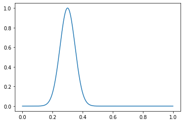
خذ بعين الاعتبار مثال دالة. قم بإنشاء توزيع عادي مع μ = 0.3 و σ = 0.05:

dist = gen_normal_distribution(0.3, 0.05, 256, max_val=1)
print(dist.max())
>>> 1.0
plt.plot(np.linspace(0, 1, 256), dist)

أعلن معلمات مجموعة البيانات لدينا:

in_distribution_size = 2000
out_distribution_size = 200
val_size = 100
sample_size = 256

random_generator = np.random.RandomState(seed=42) #    seed

ووظائف توليد الأمثلة طبيعية وغير طبيعية. تعتبر التوزيعات بحد أقصى عادي وغير طبيعي - باثنين:

def generate_in_samples(size, sample_size):
  global random_generator

  in_samples = np.zeros((size, sample_size))

  in_mus = random_generator.uniform(0.1, 0.9, size)
  in_sigmas = random_generator.uniform(0.05, 0.5, size)

  for i in range(size):
    in_samples[i] = gen_normal_distribution(in_mus[i], in_sigmas[i], sample_size, max_val=1)

  return in_samples

def generate_out_samples(size, sample_size):
  global random_generator

  #     
  out_samples = generate_in_samples(size, sample_size)

  #        
  out_additional_mus = random_generator.uniform(0.1, 0.9, size)
  out_additional_sigmas = random_generator.uniform(0.01, 0.05, size)

  for i in range(size):
    anomaly = gen_normal_distribution(out_additional_mus[i], out_additional_sigmas[i], sample_size, max_val=0.12)
    out_samples[i] += anomaly

  return out_samples

هذا ما يبدو عليه المثال العادي:

in_samples = generate_in_samples(in_distribution_size, sample_size)
plt.plot(np.linspace(0, 1, sample_size), in_samples[42])

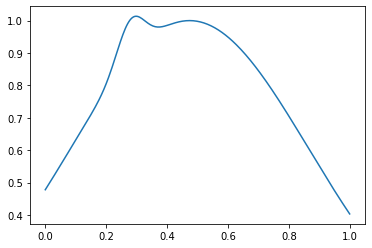
وغير طبيعي - مثل هذا:

out_samples = generate_out_samples(out_distribution_size, sample_size)
plt.plot(np.linspace(0, 1, sample_size), out_samples[42])

إنشاء صفائف مع العلامات والعلامات:

x = np.concatenate((in_samples, out_samples))
#     0,  -- 1
y = np.concatenate((np.zeros(in_distribution_size), np.ones(out_distribution_size)))

#   / 
x_train, x_test, y_train, y_test = train_test_split(x, y, test_size=0.2, shuffle=True, random_state=42)

. , , 2 1 (). , ( ), :

#     100   100  
x_val_out = generate_out_samples(val_size, sample_size)
x_val_in = generate_in_samples(val_size, sample_size)

x_val = np.concatenate((x_val_out, x_val_in))
y_val = np.concatenate((np.ones(val_size), np.zeros(val_size)))

, , Sklearn: SVM . , , .

#     
from sklearn.metrics import classification_report
from sklearn.metrics import f1_score

One class SVM

from sklearn.svm import OneClassSVM

OneClassSVM nu — .

out_dist_part = out_distribution_size / (out_distribution_size + in_distribution_size)
svm = OneClassSVM(nu=out_dist_part)
svm.fit(x_train, y_train)
>>> OneClassSVM(cache_size=200, coef0=0.0, degree=3, gamma='scale', kernel='rbf',
            max_iter=-1, nu=0.09090909090909091, shrinking=True, tol=0.001,
            verbose=False)

svm_prediction = svm.predict(x_val)
svm_prediction[svm_prediction == 1] = 0
svm_prediction[svm_prediction == -1] = 1

sklearn — classification_report, Anomaly detection , precision recall, :

print(classification_report(y_val, svm_prediction))

>>>           precision    recall  f1-score   support

         0.0       0.57      0.93      0.70       100
         1.0       0.81      0.29      0.43       100

    accuracy                           0.61       200
   macro avg       0.69      0.61      0.57       200
weighted avg       0.69      0.61      0.57       200

, . f1-score , .

Isolation forest

, , - ?

from sklearn.ensemble import IsolationForest

, . :

out_dist_part = out_distribution_size / (out_distribution_size + in_distribution_size)

iso_forest = IsolationForest(n_estimators=100, contamination=out_dist_part, max_features=100, n_jobs=-1)
iso_forest.fit(x_train)
>>> IsolationForest(behaviour='deprecated', bootstrap=False,
                contamination=0.09090909090909091, max_features=100,
                max_samples='auto', n_estimators=100, n_jobs=-1,
                random_state=None, verbose=0, warm_start=False)

Classification report? — Classification report!

iso_forest_prediction = iso_forest.predict(x_val)
iso_forest_prediction[iso_forest_prediction == 1] = 0
iso_forest_prediction[iso_forest_prediction == -1] = 1

print(classification_report(y_val, iso_forest_prediction))
>>>            precision    recall  f1-score   support

         0.0       0.50      0.91      0.65       100
         1.0       0.53      0.10      0.17       100

    accuracy                           0.51       200
   macro avg       0.51      0.51      0.41       200
weighted avg       0.51      0.51      0.41       200

RandomForestClassifier

, - " ?" , :

from sklearn.ensemble import RandomForestClassifier

random_forest = RandomForestClassifier(n_estimators=100, max_features=100, n_jobs=-1)
random_forest.fit(x_train, y_train)
>>> RandomForestClassifier(bootstrap=True, ccp_alpha=0.0, class_weight=None,
                       criterion='gini', max_depth=None, max_features=100,
                       max_leaf_nodes=None, max_samples=None,
                       min_impurity_decrease=0.0, min_impurity_split=None,
                       min_samples_leaf=1, min_samples_split=2,
                       min_weight_fraction_leaf=0.0, n_estimators=100,
                       n_jobs=-1, oob_score=False, random_state=None, verbose=0,
                       warm_start=False)

random_forest_prediction = random_forest.predict(x_val)
print(classification_report(y_val, random_forest_prediction))
>>>            precision    recall  f1-score   support

         0.0       0.57      0.99      0.72       100
         1.0       0.96      0.25      0.40       100

    accuracy                           0.62       200
   macro avg       0.77      0.62      0.56       200
weighted avg       0.77      0.62      0.56       200

Autoencoder

, : . .

, "" , . 2 : Encoder' Decoder', .

"" , , .

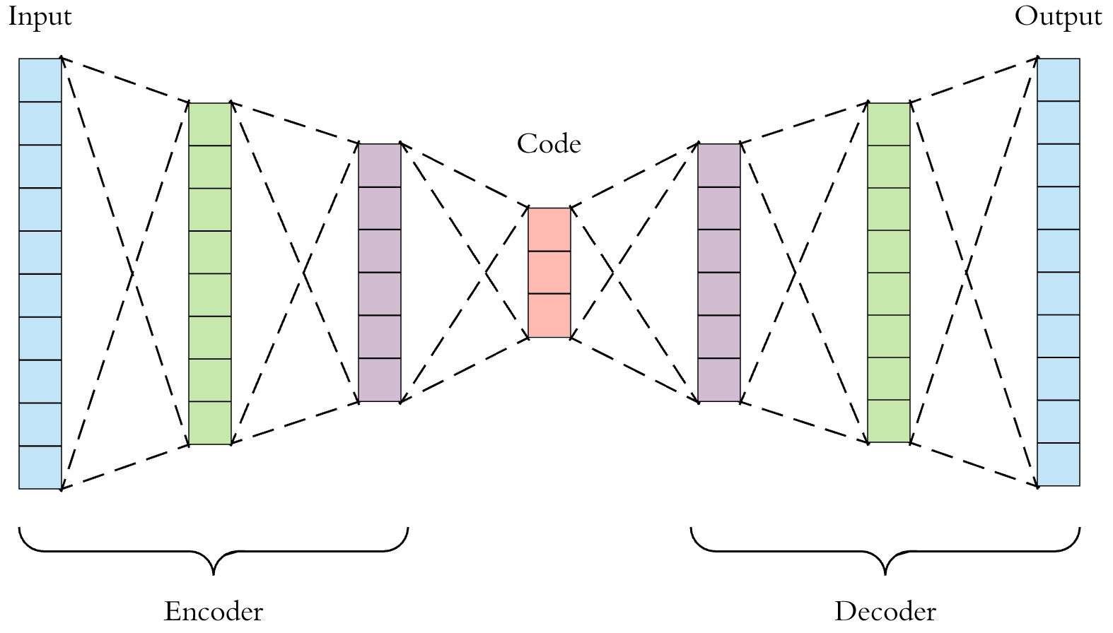
? , , , . , 9% 91% . , . , , : .

PyTorch, :

import torch
from torch import nn
from torch.utils.data import TensorDataset, DataLoader
from torch.optim import Adam

batch_size = 32
lr = 1e-3

. , , "" . , ( , learning rate, ) , , .

#      x_train,    
train_in_distribution = x_train[y_train == 0]
train_in_distribution = torch.tensor(train_in_distribution.astype(np.float32))

train_in_dataset = TensorDataset(train_in_distribution)
train_in_loader = DataLoader(train_in_dataset, batch_size=batch_size, shuffle=True)

#       ,           
test_dataset = TensorDataset(
    torch.tensor(x_test.astype(np.float32)),
    torch.tensor(y_test.astype(np.long))
)
test_loader = DataLoader(test_dataset, batch_size=batch_size, shuffle=False)

val_dataset = TensorDataset(torch.tensor(x_val.astype(np.float32)))
val_loader = DataLoader(val_dataset, batch_size=batch_size, shuffle=False)

. 4 , ( 2 : μ, — σ, ; 4 , ).

class Autoencoder(nn.Module):
  def __init__(self, input_size):
    super(Autoencoder, self).__init__()
    self.encoder = nn.Sequential(
      nn.Linear(input_size, 128),
      nn.LeakyReLU(0.2),
      nn.Linear(128, 64),
      nn.LeakyReLU(0.2),
      nn.Linear(64, 16),
      nn.LeakyReLU(0.2),
      nn.Linear(16, 4),
      nn.LeakyReLU(0.2),
    )
    self.decoder = nn.Sequential(
      nn.Linear(4, 16),
      nn.LeakyReLU(0.2),
      nn.Linear(16, 64),
      nn.LeakyReLU(0.2),
      nn.Linear(64, 128),
      nn.LeakyReLU(0.2),
      nn.Linear(128, 256),
      nn.LeakyReLU(0.2),
    )

  def forward(self, x):
    x = self.encoder(x)
    x = self.decoder(x)
    return x

model = Autoencoder(sample_size).cuda()
criterion = nn.MSELoss()
per_sample_criterion = nn.MSELoss(reduction="none") # loss   ,   
#   reduction="none" pytorch  loss'   
optimizer = Adam(model.parameters(), lr=lr, weight_decay=1e-5)

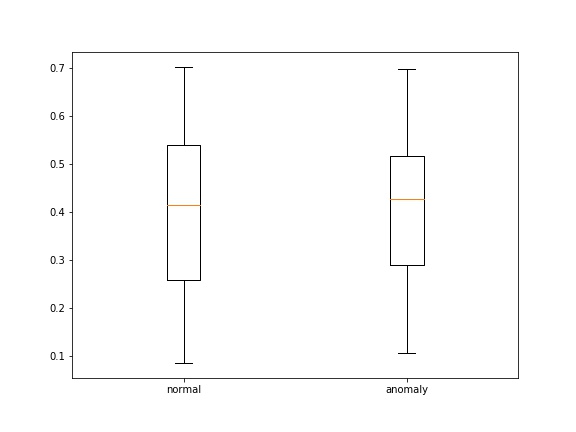
- loss' , , boxplot' :

def save_score_distribution(model, data_loader, criterion, save_to, figsize=(8, 6)):
  losses = [] #    loss    
  labels = [] #  --  
  for (x_batch, y_batch) in data_loader:
    x_batch = x_batch.cuda()

    output = model(x_batch)
    loss = criterion(output, x_batch)

    loss = torch.mean(loss, dim=1) #  loss    (        )
    loss = loss.detach().cpu().numpy().flatten()
    losses.append(loss)

    labels.append(y_batch.detach().cpu().numpy().flatten())

  losses = np.concatenate(losses)
  labels = np.concatenate(labels)

  losses_0 = losses[labels == 0] #  
  losses_1 = losses[labels == 1] #  

  fig, ax = plt.subplots(1, figsize=figsize)

  ax.boxplot([losses_0, losses_1])
  ax.set_xticklabels(['normal', 'anomaly'])

  plt.savefig(save_to)
  plt.close(fig)

experiment_path = "ood_detection" #    
!rm -rf $experiment_path
os.makedirs(experiment_path, exist_ok=True)

epochs = 100

for epoch in range(epochs):
  running_loss = 0
  for (x_batch, ) in train_in_loader:
    x_batch = x_batch.cuda()

    output = model(x_batch)
    loss = criterion(output, x_batch)

    optimizer.zero_grad()
    loss.backward()
    optimizer.step()

    running_loss += loss.item()

  print("epoch [{}/{}], train loss:{:.4f}".format(epoch+1, epochs, running_loss))

  #   
  plot_path = os.path.join(experiment_path, "{}.jpg".format(epoch+1))
  save_score_distribution(model, test_loader, per_sample_criterion, plot_path)

>>> 
epoch [1/100], train loss:8.5728
epoch [2/100], train loss:4.2405
epoch [3/100], train loss:4.0852
epoch [4/100], train loss:1.7578
epoch [5/100], train loss:0.8543
...
epoch [96/100], train loss:0.0147
epoch [97/100], train loss:0.0154
epoch [98/100], train loss:0.0117
epoch [99/100], train loss:0.0105
epoch [100/100], train loss:0.0097

100

, . , :

# ,    
def get_prediction(model, x):
  global batch_size

  dataset = TensorDataset(torch.tensor(x.astype(np.float32)))
  data_loader = DataLoader(dataset, batch_size=batch_size, shuffle=False)

  predictions = []
  for batch in data_loader:
    x_batch = batch[0].cuda()
    pred = model(x_batch) # x -> encoder -> decoder -> x_pred
    predictions.append(pred.detach().cpu().numpy())

  predictions = np.concatenate(predictions)
  return predictions

#      (  )
def compare_data(xs, sample_num, data_range=(0, 1), labels=None):
  fig, axes = plt.subplots(len(xs))
  sample_size = len(xs[0][sample_num])

  for i in range(len(xs)):
    axes[i].plot(np.linspace(*data_range, sample_size), xs[i][sample_num])

  if labels:
    for i, label in enumerate(labels):
      axes[i].set_ylabel(label)

x_test_pred = get_prediction(model, x_test)
compare_data([x_test[y_test == 0], x_test_pred[y_test == 0]], 10, labels=["real", "encoded"])

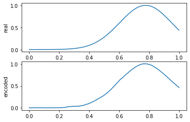
X? .

Difference score

— . , , , . .

def get_difference_score(model, x):
  global batch_size

  dataset = TensorDataset(torch.tensor(x.astype(np.float32)))
  data_loader = DataLoader(dataset, batch_size=batch_size, shuffle=False)

  predictions = []
  for (x_batch, ) in data_loader:
    x_batch = x_batch.cuda()
    preds = model(x_batch)
    predictions.append(preds.detach().cpu().numpy())

  predictions = np.concatenate(predictions)

  #     
  return (x - predictions)

from sklearn.ensemble import RandomForestClassifier

test_score = get_difference_score(model, x_test)

score_forest = RandomForestClassifier(max_features=100)
score_forest.fit(test_score, y_test)
>>> RandomForestClassifier(bootstrap=True, ccp_alpha=0.0, class_weight=None,
                       criterion='gini', max_depth=None, max_features=100,
                       max_leaf_nodes=None, max_samples=None,
                       min_impurity_decrease=0.0, min_impurity_split=None,
                       min_samples_leaf=1, min_samples_split=2,
                       min_weight_fraction_leaf=0.0, n_estimators=100,
                       n_jobs=None, oob_score=False, random_state=None,
                       verbose=0, warm_start=False)

, : 2 — . , 2 : , — difference_score, — . , , .

? . difference_score , ( ) , , . , , difference_score , ( ). .

val_score = get_difference_score(model, x_val)
prediction = score_forest.predict(val_score)
print(classification_report(y_val, prediction))
>>>            precision    recall  f1-score   support

         0.0       0.76      1.00      0.87       100
         1.0       1.00      0.69      0.82       100

    accuracy                           0.84       200
   macro avg       0.88      0.84      0.84       200
weighted avg       0.88      0.84      0.84       200

. :

indices = np.arange(len(prediction))
#       ,     
wrong_indices = indices[(prediction == 0) & (y_val == 1)]

x_val_pred = get_prediction(model, x_val)
compare_data([x_val, x_val_pred], wrong_indices[0])

? :

plt.imshow(val_score[wrong_indices], norm=Normalize(0, 1, clip=True))

plt.imshow(val_score[(prediction == 1) & (y_val == 1)], norm=Normalize(0, 1, clip=True))

plt.imshow(val_score[(prediction == 0) & (y_val == 0)], norm=Normalize(0, 1, clip=True))

, : .

Difference histograms

. . — , "", .

, difference score

print("test score: [{}; {}]".format(test_score.min(), test_score.max()))
>>> test score: [-0.2260764424351479; 0.26339245919832344]

, :

def score_to_histograms(scores, bins=10, data_range=(-0.3, 0.3)):
  result_histograms = np.zeros((len(scores), bins))

  for i in range(len(scores)):
    hist, bins = np.histogram(scores[i], bins=bins, range=data_range)
    result_histograms[i] = hist

  return result_histograms

test_histogram = score_to_histograms(test_score, bins=10, data_range=(-0.3, 0.3))
val_histogram = score_to_histograms(val_score, bins=10, data_range=(-0.3, 0.3))

plt.title("normal histogram")
plt.bar(np.linspace(-0.3, 0.3, 10), test_histogram[y_test == 0][0])

plt.title("anomaly histogram")
plt.bar(np.linspace(-0.3, 0.3, 10), test_histogram[y_test == 1][0])

, "", .

histogram_forest = RandomForestClassifier(n_estimators=10)
histogram_forest.fit(test_histogram, y_test)
>>> RandomForestClassifier(bootstrap=True, ccp_alpha=0.0, class_weight=None,
                       criterion='gini', max_depth=None, max_features='auto',
                       max_leaf_nodes=None, max_samples=None,
                       min_impurity_decrease=0.0, min_impurity_split=None,
                       min_samples_leaf=1, min_samples_split=2,
                       min_weight_fraction_leaf=0.0, n_estimators=10,
                       n_jobs=None, oob_score=False, random_state=None,
                       verbose=0, warm_start=False)

val_prediction = histogram_forest.predict(val_histogram)
print(classification_report(y_val, val_prediction))
>>>            precision    recall  f1-score   support

         0.0       0.83      0.99      0.90       100
         1.0       0.99      0.80      0.88       100

    accuracy                           0.90       200
   macro avg       0.91      0.90      0.89       200
weighted avg       0.91      0.90      0.89       200

— . , , , , . () .

— . ? VAE, ( 4 ) . . CVAE, - . , , , ..

GAN', (), . ( ).

, , .

Statistical parametric

GMM — Gaussian mixture modelling + Akaike or Bayesian Information Criterion
HMM — Hidden Markov models
MRF — Markov random fields
CRF — conditional random fields

Robust statistic

minimum volume estimation
PCA
estimation maximisation (EM) + deterministic annealing
K-means

Non-parametric statistics

histogram analysis with density estimation on KNN
local kernel models (Parzen windowing)
vector of feature matching with similarity distance (between train and test)
wavelets + MMRF
histogram-based measures features
texture features
shape features
features from VGG-16
HOG

Neural networks

self organisation maps (SOM) or Kohonen's
Radial Basis Functions (RBF) (Minhas, 2005)
LearningVector Quantisation (LVQ)
ProbabilisticNeural Networks (PNN)
Hopfieldnetworks
SupportVector Machines (SVM)
AdaptiveResonance Theory (ART)
Relevance vector machine (RVM)

, Data science' . Computer vision, . ( — !) — FARADAY Lab. — , .

Python Anomaly Detection باستخدام Autoencoders في Python